


|
|
|
|
|
|
|
|
|
|
Announcements
|
 A. Hertzmann and K. Perlin |
About CSC320
This course serves as an introduction to image analysis and image synthesis. We introduce topics from digital image processing, computer vision, non-photorealistic rendering, and computational photography. The focus is on techniques for digital special effects and on image understanding. We cover mathematical and computational methods used in computer vision and image processing. We use the Python NumPy/SciPy stack for visual computing. Students should be comfortable with calculus and linear algebra.
Course outline
Matching image patches in image space. Image filters and convolution. Aliasing. Image upsampling, image downsampling, Gaussian pyraminds, and image interpolation. Image gradients and edge detection in images. Principal Component Analysis (PCA) and applications of PCA for object detection and recognition. Fourier transforms of images and image analysis in the frequency domain. Image matting, image blending and image compositing. Image warping and image morphing. Colour in images. Introduction to machine learning for computer vision and computational photography. Introduction to recent work in computational photography.
Required math background
Here's (roughly) the math that you need for this course. Linear Algebra: vectors: the dot product, vector norm, vector addition and subtraction (geometrically and algebraically); orthogonality; projection of vectors; matrices: matrix multiplication, eigenvalues and eigenvectors, bases; linear equations. Calculus: derivatives, derivatives as the slope of the function; integrals, integrals as the area under the curve. Other topics will be needed, but are not part of the pre-requisites, so I will devote an appropriate amount of lecture time to them.
Teaching team
Instructor: Michael Guerzhoy. Office: BA4262, Email: guerzhoy at cs.toronto.edu (please include CSC320 in the subject, and please ask questions on Piazza if they are relevant to everyone.)
Getting help
Michael's office hours: Monday 4:30-6:00, Tuesday 3-4, Thursday 6-7. Or email for an appointment. Or drop by to see if I'm in. Feel free to chat with me after lecture.
Lectures and Tutorials
L0101/L2001: MW2-3 in SS2110 (sometimes also F2 in SS2110). Tutorials F2 in BA2175 (even student numbers) and BA2185 (odd student numbers).
L5101/L2501: W6-8 in BA1210 (sometimes also W8 in BA1210). Tutorials W8 in BA2175 (even student numbers) and BA2185 (odd student numbers)
Software
We will be using the Python NumPy/SciPy stack in this course. It is installed on CDF, and you can download the Anaconda distribution to your own computer. I recommend the IEP IDE available with Pyzo. To run IEP on CDF, simply type iep in the command line. We will be using Python 2. In IEP (or any other IDE), you should set the Python shell be the Anaconda executable (still called Python, but located in the Anaconda folder (on Macs, [anaconda folder]/bin)), not the default Python installed on your system
Textbooks
Computer Vision: Algorithms and Applications by Richard Szeliski covers most of the topics from the course. (Available for free on the web from the author.)
Programming Computer Vision with Python by Jan Erik Solem contains useful examples when getting started with visual computing in Python. (Available for free on the web from the author.)
Computer Vision: A Modern Approach by David Forsyth and Jean Ponce is a good advanced text.
Python Scientific Lecture Notes by Valentin Haenel, Emmanuelle Gouillart, and Gaël Varoquaux (eds) contains material on NumPy and image processing using SciPy. (Free on the web.)
Digital Image Processing by Ken Castleman is an additional reference.
Evaluation
35%: Programming projects
The better of: [10%: Midterm Exam, 55% Final Exam], [30%: Midterm Exam, 35%: Final Exam]
You must receive at least 40% on the final exam to pass the course.
Final Exam
Time and location: shown here.
Format: basically similar to the midterm and to previous years' exams.
Coverage: The lectures and the projects. You should have complete understanding of all the core algorithms. For special topics (flash/no-flash and dark flash photography, Eulerian motion magnification, face beautification) you're only responsible for what's in the study guide, and for understanding the goals of the algorithms and the approximate strategy that's used
Study guide (updated continuously (final update: Apr. 2)): here. Student-curated Google doc with some solutions: here.
Midterm
Feb 27, 4pm-6pm in ES 1050 (Make-up midterm for those who have a documented (a screenshot and/or explanatory email is sufficient) conflict with the main timeslot: 6pm-8pm on the same day, location TBA.).
Coverage: the lectures and the projects, focusing on the lectures.
The study guide. These are just questions I came up with by going through the slides. Similar questions will appear on the midterm, though the midterm questions are unlikely to be that open-ended. There may also be questions about the projects. There are past exams and midterms here. I rearranged the topics, so look at the final exams and practice questions, and pick the questions which are relevant to our topics.
Projects
A sample report/LaTeX template containing advice on how to write CSC320 reports is here (see the pdf and tex files). (The example is based on Programming Computer Vision, pp27-30.) Key points: your code should generate all the figures used in the report; describe and analyze the inputs and the outputs; add your interpretation where feasible.
Project 1 (8%): The Prokudin-Gorskii Colour Photo Collection (due: Jan. 24 at 11PM)
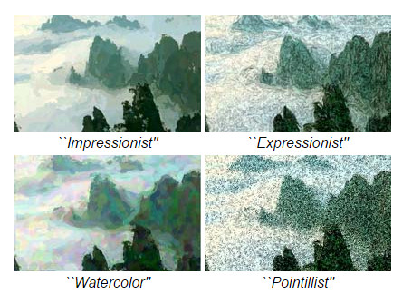
Project 2 (10%): Painterly Rendering (due: Feb.2123 at 11PM, no late submissions after 1AM on Tuesday.) NEW: results gallery
Project 3 (10%): Face Recognition and Classification with Eigenfaces (due: Mar.2021 at 11PM)
Project 4 (7%): Triangulation Matting (due: Mar.2830 at 11PM, no late submissions after Mar. 31 1AM)
Lateness penalty: 10% of the possible marks per day, rounded up. Projects are only accepted up to 48 hours after the deadline.The projects will be submitted and graded using MarkUs. You should be able to login to MarkUs starting from the second week of classes.
The projects are to be done by each student or team alone. Any discussion of the projects with other students should be about general issues only, and should not involve giving or receiving written, typed, or emailed notes. Please refer to François Pitt's Guidelines for Avoiding Plagiarism.
Lecture notes
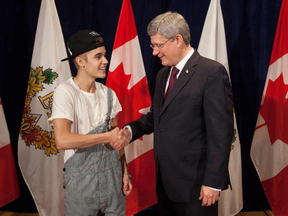
Week 1: Intro, Matching with SSD, NCC, etc. slides. matching patches (UPDATED 8/1/2014). basic_numpy.py (the bieber.jpg file I used).
Just for fun: Vermeer took manual photos!, The Science of Art.
Q: Isn't it inefficient to do detection with a sliding window, where we have to look at every possible window in the image and compare it to the reference patch? A1: Yes, on a non-parallel computer. That suggests that the brain does similar task in parallel. A2: Yes, that's why we need to do the matching on an appropriate scale -- scale the image to a smaller one. A3: Yes, that's why we may need to detect interest points on the image first. A4: Maybe yes, but sliding window detection is actually used in practical applications: any face detection application you see likely uses a sliding window.
Why is it that you can only barely see see the maple leaf on the red channel of the Bieber photo? Because the red channel is close to 255 for the red flag, so it shows as white on the red channel of the photo.
Week 2: contrast.py, Aliasing and Filters, part I (Reading: Szeliski 3.1, 2.3.1, 3.2.1-3.2.2), Filters, anti-aliasing, convolution, noise, downsampling, Guassian pyramids
As mentioned in lecture, the Guassian noise in low-exposure (high-shutter speed) photos is caused by thermal noise (the link is just for fun). What causes salt-and-pepper noise? Black pixels could be "dead pixels" (broken sensor, etc.); white pixels in astronomical images could be cosmic rays.
Photography basics: shutter speed, low-exposure photos, etc. from Improve Photography and Photography Hero.
Q in class: can't we get rid of Gaussian noise without blurring the image? A: If we don't know anything about the image, then no. If we know something about what's in the image, then we can use that information. More in the next few weeks
Just for fun (briefly mentioned in class): error detection and correction makes miscommunicating pixels over networks less likely.
Week 3: Edge Detection lecture (reading: Wikipedia seems to be better than the textbook on this, though not perfect; also see Allan Jepson's notes on edge detection). Gradient write-up, partial derivatives and the gradient at Khan Academy, Understanding the Gradient
Just for fun: Q in lecture: if we know the original image, and can see the filtered image, can we figure out what the filter was? A1: Yes, if we know what the filter generally looks like (e.g., we know it's a Gaussian filter), we can figure out the parameters (the sigma for the Guassian filter) by solving a system of equations. A2: If the filtering is noisy and we don't know what the filter looks like generally, than that's a much harder problem. A related problem is deconvolution, obtaining the original image from the filtered image. Here's a cool paper by UofT/NYU/MIT researchers about addressing the problem where the filtered image is one that's produced by shaking the camera.
Visualizing functions of two variables as surfaces
Just for fun: computing partial derivatives (in particular, e.g., fixing the y and computing the derivative with respect to x) is conceptually similar to partial application in programming languages (see also p. 60 in David Liu's notes).
Just for fun: Amazon Mechanical Turk is used in computer vision R&D to, for example, manually label boundaries between objects
Mentioned in passing in response to a question (so no need to remember the details): Connected-component labeling
Tutorial: Filters and Noise (edge.png)
Week 4: Interpolation and upsampling. Linear interpolation and bilinear interpolation on Wikipedia. (Nearest-neighbour, linear, and bilinear interpolation were done on the blackboard in class.)
Demo for span, linear dependence, and linear independence (UPDATED Jan. 30 so that the points in the plot are colour-coded according to the coefficients of the vectors)
The linear algebra reviewed: linear dependence and independence, span, (orthonormal) bases, dimension, projection onto subspaces. Khan academy link. The material is standard, and is in any MAT223 textbook as well.
PCA and Eigenfaces. Reading for PCA/Eigenfaces: 14.2.1 of Szeliski, Allan Jepson and David Fleet's notes (these are notes for the graduate vision class; skip the derivations and proofs of theorems.) See also this lecture by Pedro Domingos.
Just for fun: average faces are more attractive. (But not the most attractive.) Note: Galton's original method of averaging faces is just computing the mean faces pixelwise.Week 5: PCA, part II, denoising with PCA.
The Frequency Domain (updated Feb. 4) (up to slide 27). Reading: An Intuitive Explanation of Fourier Theory by Steven Lehar, Introduction to Fourier Transforms for Image Processing by John Brayer, Sections 3.4-3.5 in Szeliski + the websites about the FT linked in the slides.
Some code for visualizing gratings., code for computing the DFT of images (to be covered next week).
Tutorial: canny.py from P2 and Canny edges.
Midterm preview: some questions will test recall (e.g., "give the pseudocode for simulating Gaussian noise in an image"). Some questions will ask for some analysis of formulas (e.g., "in Project 1, you were asked to compute the SSD between two images. One way to compute the SSD between two images which don't overlap completely is to assume that for image I, I(i,j)=0 if the point (i,j) is not inside the image. Why is that a bad idea, and what would happen if you were to try to align images that way? What's a better way of handling the issue of computing the SSD for images which don't completely overlap?." "Suppose we have a wheel with four spokes rotating at 5 revolutions per second clockwise. We take a photo of the wheel every X milliseconds, and compose a movie out of the photos. In the movie, the wheel appears to be rotating counterclockwise. Give a value of X for which this would happen." How to study: go through the slides, and make sure that you understand what the point of every slide is. Try to come up with analysis questions like the ones above, and try to answer them. Go through the code posted, and make sure you understand what every line does. For Fourier Transforms (which we haven't finished yet): detailed understanding of the integrals is not essential. Understanding the 2D DFT completely is important. Note on the readings: you are only responsible for what was done in class, although the readings should help you with studying the things that were done in class.
There are past exams and midterms here. I rearranged the topics, so look at the final exams and practice questions, and pick the questions which are relevant to our topics.
Just for fun, coded up on request during the break in the evening section: how to make an image look like it was taken through a red filter? redfilter.py (grumpy.jpg).
Week 6: (Related to Project 2) line_drawing.py (Just for fun: aliasing in line drawing).
The Frequency Domain (cont'd). Some code for visualizing gratings (meshgrid documentation.)
Reading: continue the readings from last week. Unsharp masking.
Just for fun: Mona Lisa's Smile. The original note in Science. (Other theories about the Mona Lisa smile.)
Michael Kamm's amazingly good hybrid images. The hybrid images on the webpage of the inventor of hybrid images, Aude Oliva.
Week 7: Blending and compositing, Face Recognition with PCA
Question in class: can we construct a Gaussian pyramid without downsampling? A (short write-up, talk to me for more detail): First, let's figure out what repeated convolution with a Gaussian means. In Fourier domain, that's just multiplying Guassian together. In Fourier domain, multiplying G(1/sigma1^2)G(1/sigma2^2) gives G(1/(sigma1^2+sigma2^2)), so the convolution of two Gaussians G(sigma1^2) and G(sigma2^2) is G(sigma1^2+sigma2^2). If I2 is the downsampled version of I (by a factor of two), smoothing it with G(sigma) is the same as sommething the original image with G(2*sigma). So we are smoothing the image successively using G(2), G(4), G(8), ... . At the k-th step, we are smoothing using G(sqrt(2^2+4^2+8^2+...+(2^(2k)))). Try this to see that this works.
Just for fun: blurred video, non-blurred video from Antonio Torralba.
Week 8: Мatting. Solving systems of linear equations with NumPy. The original Triangulation Matting paper. Reading: Section 10.4.1 of Szeliski.
We went over the midterm (except for the last question)
Just for fun: Chroma keying (with links to explanations of how this used to be done in film without digital image processing).
Coming up: Section 3.6 of Szeliski.
Week 9: Matting equation: C = a*F+(1-a)*B. Suppose we know C and B. How to transform this into a linear equation?
F + (B-C)*(1/a) = B
This is obtained by rearranging the terms, and can be written in matrix form, with F and (1/a) as the unknowns.
Separating the dataset into training, test, and validation sets. Optional watching (more advanced than what we did): Andrew Ng's coursera segment on cross-validation.
Just for fun: Q in lecture: how do we determine what the size of the test set should be? A: in general in academic research in computer vision, the dataset comes with a standard test set, so that's what you use. In general, the performance on the test set is an estimate for the performance on new real-world data. The larger the test set, the more precise is this estimate. If the output is binary (e.g., face/not a face), the precision of the estimate could be said to be 100%/sqrt(N), where N is the size of the test set. For example, if the performance on a test set of size 1000 for face/non face classification is 80%, then the performance on real world data can be expected to be within about 100%/sqrt(1000)=3% of 80% (i.e., between 77% and 83%). (This estimate is obtained by computing the standard error for the ratio estimator. For more details, talk to me or take e.g. STA304.)
Image warping (up to backward/forward warps). Reading: Szeliski Section 3.6.
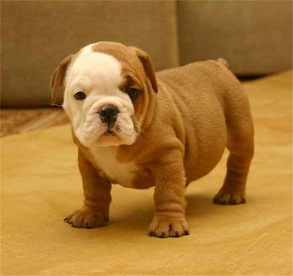
Week 10: Image warping (to the end), image warping code (puppy.jpg). Reading: Szeliski Section 3.6.
Image morphing (PPT with animations). 500 Years of Female Portraits in Western Art, 0 to 65 and back in a minute.
Just for fun: perspective in art, perspective in the works of Paul Cézanne.
Week 11: (Started on the Friday of week 10 for the day section) A brief intro to imaging and colour, colour balancing. Reading: Szeliski 2.3.2.
An illustration: #thedress
Flash/no flash and dark flash photography. Homepages: Dark Flash Photography at New York University, Flash/No-Flash Photography at Microsoft Research.
Eulerian motion magnification (PPTX). Homepages: Eulerian Video Magnification for Revealing Subtle Changes in the World at MIT, Video Magnification at MIT. Video: Eulerian Video Magnification.
Week 12: Machine learning for visual computing. Just for fun: TED talk on object recognition with Deep Learning by Fei-Fei Li (Stanford).
Big Data for photo completion. Homepage: Scene Completion Using Millions of Photographs at Carnegie Mellon University.
Data-Driven Beautification. Homepage: Digital Face Beautification, YouTube clip.
Morphing review (these are just extracted from the warping and morphing lectures.)
See you in office hours and at the exam, and thanks for a great semester!
MarkUs
All project submission will be done electronically, using the MarkUs system. You can log in to MarkUs using your CDF login and password.
To submit as a group, one of you needs to "invite" the other to be partners, and then the other student needs to accept the invitation. To invite a partner, navigate to the appropriate Assignment page, find "Group Information", and click on "Invite". You will be prompted for the other student's CDF user name; enter it. To accept an invitation, find "Group Information" on the Assignment page, find the invitation listed there, and click on "Join". Only one student must invite the other: if both students send an invitation, then neither of you will be able to accept the other's invitation. So make sure to agree beforehand on who will send the invitation! Also, remember that, when working in a group, only one person must submit solutions.
To submit your work, again navigate to the appropriate Exercise or Assignment page, then click on the "Submissions" tab near the top. Click "Add a New File" and either type a file name or use the "Browse" button to choose one. Then click "Submit". You can submit a new version of any file at any time (though the lateness penalty applies if you submit after the deadline) — look in the "Replace" column. For the purposes of determining the lateness penalty, the submission time is considered to be the time of your latest submission.
Once you have submitted, click on the file's name to check that you have submitted the correct version.
LaTeX
Web-based LaTeX interfaces: WriteLaTeX, ShareLaTeX
TeXworks, a cross-platform LaTeX front-end. To use it, install MikTeX on Windows and MacTeX on Mac
Detexify2 - LaTeX symbol classifier
The LaTeX Wikibook.
Additional LaTeX Documentation, from the home page of the LaTeX Project.
Policy on special consideration
Special consideration will be given in cases of documented and serious medical and personal cirumstances.
Previous offerings of CSC320