Lecture 06: Recurrences 2
2025-06-04
Recurrences 2
Recap
Recurrences
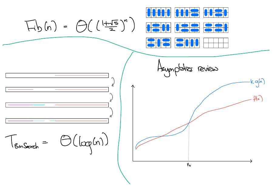
Last time, we used induction to prove asymptotic bounds on recursive functions. For example, we showed that. \[ \mathrm{Fib}(n) = \Theta(\varphi^n), \]
and \[ T_\mathrm{BinSearch}(n) = \Theta(\log(n)). \]
Last time’s approach
Last time, the process looked like
- Guess an upper bound.
- Try to prove the upper bound.
- Try to prove a tighter upper bound or a matching lower bound.
Here are two weaknesses to this approach.
- What if you get unlucky with your guess?
- The proofs were slow, technical and not incredibly intuitive.
Today’s approach
Today, we will see how to
- Remove technical details.
- Make better guesses.
- Streamline the process for solving certain types of recurrences.
Technicalities
Technicalities - Base Cases
The base case typically involves calculating some values of the recursive function and selecting constants that are large enough so that the calculations work out.
The base usually works out and is a little tedious to check, so for the rest of this class, you may skip this step, as long as you swear the following oath.
I swear that I understand that a full proof by induction requires a base case
Technicalities - Floors and Ceilings
In divide-and-conquer algorithms, we typically split the problem into subproblems of roughly equal size. For example, we might split a problem of size \(n\) into 2 sub-problems of size \(n/2\). When \(n\) is not divisible by 2, this is one subproblem of \(\left\lfloor n/2 \right\rfloor\) and another of \(\left\lceil n/2 \right\rceil\).
However, replacing \(\left\lceil n/2 \right\rceil\) and \(\left\lfloor n/2 \right\rfloor\) with \(n/2\) has a negligible impact on the asymptotics, so we can just ignore floors and ceilings. See Introduction To Algorithms (CLRS), section 4.62 for a discussion on this.
The substitution method
The substitution method for solving recurrences is proof by (complete) induction with the simplifications applied.
The substitution method
- Remove all floors and ceilings from recurrence \(T\).
- Make a guess for \(f\) such that \(T(n) = O(f(n))\).
- Write out the recurrence: \(T(n) = ...\).
- Whenever \(T(k)\) appears on the RHS of the recurrence, substitute it with \(cf(k)\).
- Try to prove \(T(n) \leq cf(n)\).
- Pick \(c\) to make your analysis work!
The substitution method
- If you want to show \(T = \Theta(f)\), you also need to show \(T(n) = \Omega(f(n))\). This is the same as steps 3-6, where the \(\leq\) in step 5 is replaced by a \(\geq\).
You can also add as many lower-order terms as you want. I.e. you can show \(T(n) = cf(n) + d\).
- The constant \(c\) that you pick when trying to show \(T = \Omega(f)\) can be different from the constant that you picked when trying to show \(T = O(f)\).
Today’s approach
\(T_\mathrm{BinSearch}(n) = T_\mathrm{BinSearch}({\color{red} n/2}) + 1\)
Claim. \(T_\mathrm{BinSearch}(n) = O(\log(n))\).
Solution
Use the substitution method. \[ \begin{align*} T_\mathrm{BinSearch}(n) & = T_\mathrm{BinSearch}(n/2) + 1 \\ & \leq c\log(n/2) + 1 \\ & = c(\log(n) - \log(2)) + 1 \\ & = c\log(n) - c + 1, \end{align*} \]
which is at most \(c\log(n)\) when \(c \geq 1\).
Merge Sort
The Sorting Problem
Input. A list \(l\).
Output. \(l\), but sorted.
Let’s think of \(l \in \mathrm{List}[\mathbb{N}]\), i.e. \(l\) is a list of natural numbers is sorted iff \(i \leq j \implies l[i] \leq l[j]\).
In general, sorting makes sense for \(l \in \mathrm{List}(A)\), as long as the elements of \(A\) can be ordered.
Merge Sort - Code
Screenshots of Code
def merge_sort(l):
    n = len(l)
    if n <= 1:
        return l
    else:
        left = merge_sort(l[:n//2]) # Sort the left subarray
        right = merge_sort(l[n//2:]) # Sort the right subarray
        return merge(left, right) # Merge the sorted subarrays
def merge(l1, l2):
"""
Input: sorted lists: l1, l2
Output: l, a sorted list of elements from both l1 and l2
"""
l = []
while True:
# If either list is empty, concatenate the other list to the end and return
if len(l1) == 0:
return l + l2
if len(l2) == 0:
return l + l1
# Otherwise, both lists are non-empty, so append the smallest element in either list
if l1[0] <= l2[0]:
l.append(l1.pop(0)) # pop(0) retrives first element and removes it from the list
else:
l.append(l2.pop(0)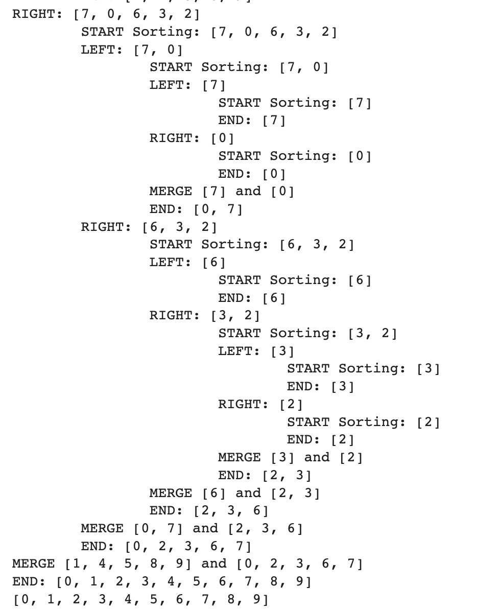
Merge Sort Complexity
def merge_sort(l):
n = len(l)
if n <= 1:
return l
else:
left = merge_sort(l[:n//2]) # Sort the left subarray
right = merge_sort(l[n//2:]) # Sort the right subarray
return merge(left, right) # Merge the sorted subarrays\[ T_\mathrm{MS}(n) = 2T_\mathrm{MS}(n/2) + T_{\mathrm{Merge}}(n) \]
Merge Complexity
def merge(l1, l2):
    """
    Input: sorted lists: l1, l2
    Output: l, a sorted list of elements from both l1 and l2
    """
    l = []
    while True:
        # If either list is empty, concatenate the other list to the end and return
        if len(l1) == 0:
            return l + l2
        if len(l2) == 0:
            return l + l1

        # Otherwise, both lists are non-empty, so append the smallest element in either list
        if l1[0] <= l2[0]:
            l.append(l1.pop(0)) # pop(0) retrives first element and removes it from the list
        else:
l.append(l2.pop(0)Let \(n\) be the total number of elements in l1 and l2. What is the complexity of merge in terms of \(n\)?
Solution
\(\Theta(n)\). Explanation: Each iteration of the while loop adds at least one element to the merged list.
Merge Sort Complexity
def merge_sort(l):
    n = len(l)
    if n <= 1:
        return l
    else:
        left = merge_sort(l[:n//2]) # Sort the left subarray
        right = merge_sort(l[n//2:]) # Sort the right subarray
        return merge(left, right) # Merge the sorted subarrays
\[ T_\mathrm{MS}(n) = 2T_\mathrm{MS}(n/2) + n \]
Recurrences as Sums
\(T_\mathrm{MS}(n) = 2T_\mathrm{MS}(n/2) + n\)
\[ \begin{align*} T_\mathrm{MS}(n) & = 2T_\mathrm{MS}(n/2) + n \\ & = 2(2T_\mathrm{MS}(n/4) + n/2) + n \\ & = 4T_\mathrm{MS}(n/4) + 2n \\ & = 4(2T_\mathrm{MS}(n/8) + n/4) + 2n \\ & = 8T_\mathrm{MS}(n/8) + 3n \\ & = 8(2T_\mathrm{MS}(n/16) + n/8) + 3n \\ & = 16T_\mathrm{MS}(n/16) + 4n \\ ... \end{align*} \]
Let’s say \(n = 2^k\) for some \(k\). Then eventually, we get to... \[ T_\mathrm{MS}(n) = 2^kT_\mathrm{MS}(n/2^k) + kn = nT_\mathrm{MS}(1) + kn = \Theta(n\log(n)) \]
Recursion Trees
Recursion Trees are a great way to visualize the sum.
Recursion Trees
\(T_\mathrm{MS}(n) = 2T_\mathrm{MS}(n/2) + n\)
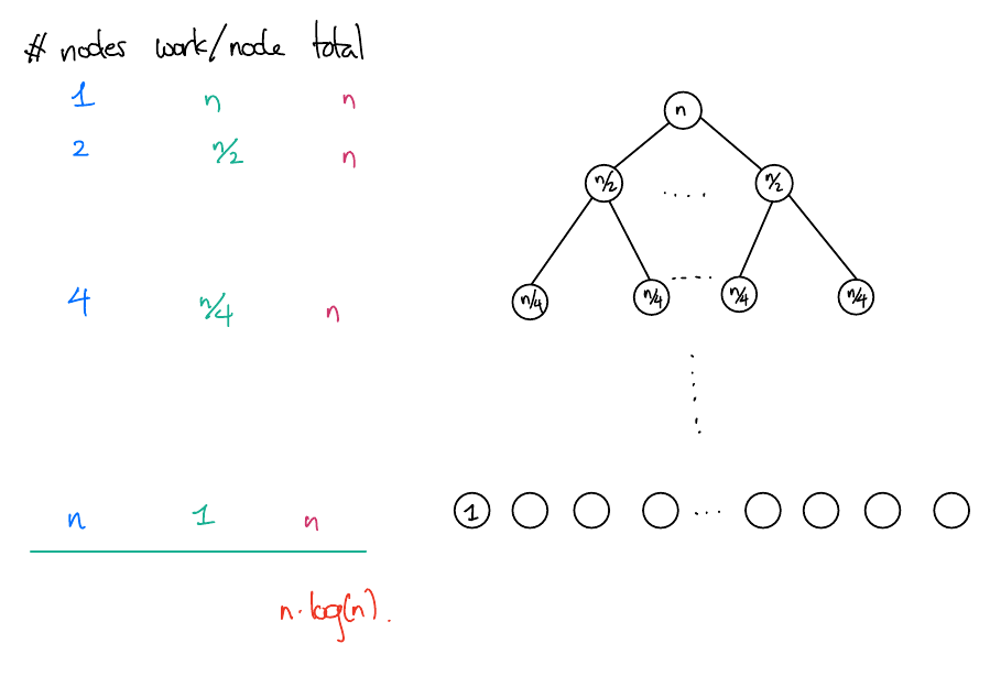
Using recursion trees
Like in the previous example, we can sometimes use the recursion tree to compute the runtime directly.
Other times, we won’t be able to compute the runtime directly, but we can still use recursion trees to make a good guess. We can then prove our guess was correct using the substitution method.
\(T(n) = T(n/3) + T(2n/3) + n\)
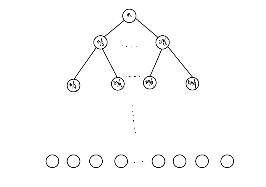
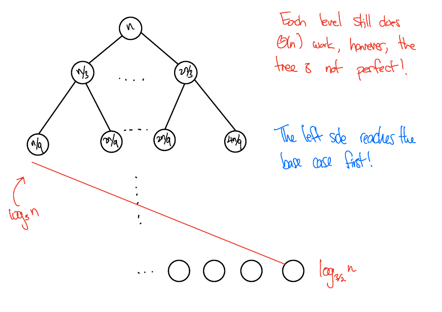
Lower bound: Remove all nodes with height \(> \log_3(n)\). The remaining tree is perfect, has height \(\log_3(n)\), and \(n\) work at each level. So guess \(n\log(n)\).
Upper bound: Imagine levels below \(\log_3(n)\) also do \(n\) work. In this case, we do \(n\) work for \(\log_{3/2}(n)\) levels, so again guess \(n \log(n)\).
Prove the guess using the substitution method (exercise).
The Master Theorem
Standard Form Recurrences
A recurrence is in standard form if it is written as
\[ T(n) = aT(n/b) + f(n) \]
For some constants \(a \geq 1\), \(b > 1\), and some function \(f:\mathbb{N}\to \mathbb{R}\).
Most divide-and-conquer algorithms will have recurrences that look like this.
Thinking about the parameters
\[ T(n) = aT(n/b) + f(n) \]
- \(a\) is the branching factor of the tree - how many children does each node have?
- \(b\) is the reduction factor - how much smaller is the subproblem in the next level of the tree compared to this level?
- \(f(n)\) is the non-recursive work - how much work is done outside of the recursive call on inputs of size \(n\)? Again, we make the assumption that \(f\) is positive and non-decreasing.
Recursion tree for standard form recurrences
Draw a recursion tree for the standard form recurrence. In terms of \(a, b, f\)...
- What is the height of the tree?
- What is the number of vertices at height \(h\)?
- What is the subproblem size at height \(h\)?
- What is the total non-recursive work at level \(h\)?
Solution
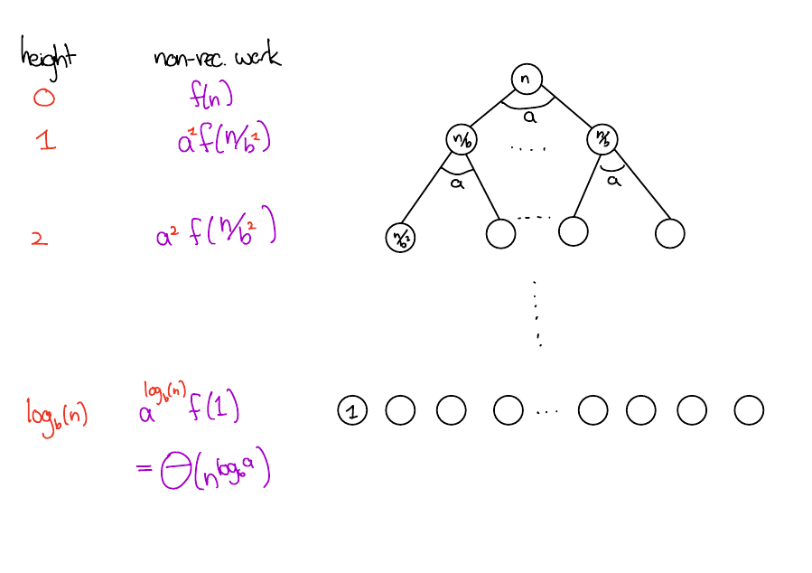
Summary
The height of the tree is \(\log_b(n)\)
The number of vertices at level \(h\) is \(a^h\)
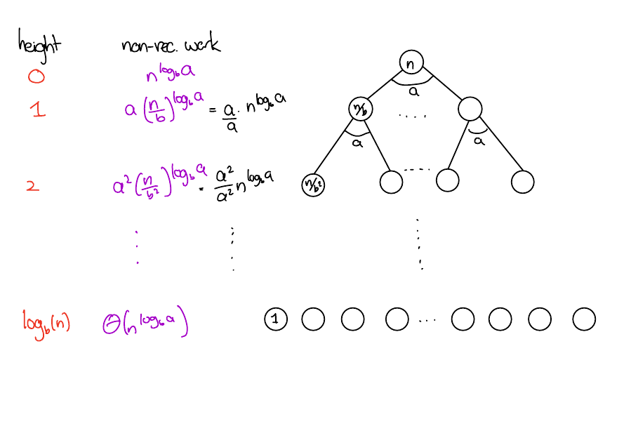
The total non-recursive work done at level \(h\) is \(a^hf(n/b^h)\). Of note are
- Root work. \(f(n)\)
- Leaf work. \(a^{\log_b(n)}\cdot f(1) = \Theta(n^{\log_b(a)})\). (see here for details)
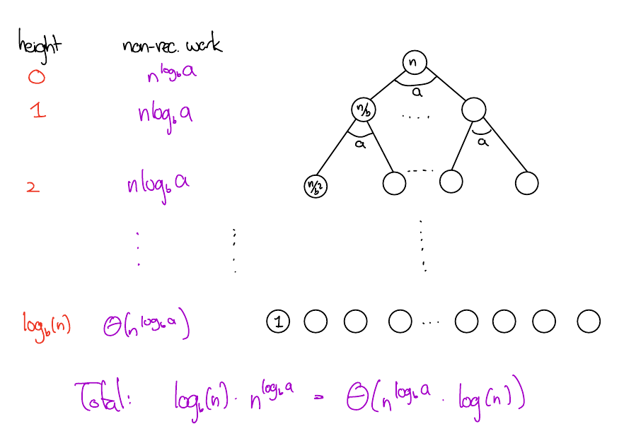
Summing up the levels, the total amount of work done is
\[ \sum_{h = 0}^{\log_b(n)}a^hf(n/b^h). \]
The Master Theorem
The Master Theorem is a way to solve most standard form recurrences quickly.
We get the Master Theorem by analyzing the recursion tree for a generic standard form recurrence.
The Master Theorem
Let \(T(n) = aT(n/b) + f(n)\). Define the following cases based on how the root work compares with the leaf work.
Leaf heavy. \(f(n) = O(n^{\log_b(a) - \epsilon})\) for some constant \(\epsilon > 0\).
Balanced. \(f(n) = \Theta(n^{\log_b(a)})\)
Root heavy. \(f(n) = \Omega(n^{\log_b(a) + \epsilon})\) for some constant \(\epsilon > 0\), and \(af(n/b) \leq cf(n)\) for some constant \(c < 1\) for all sufficiently large \(n\).
Then,
\[ T(n) = \begin{cases} \Theta(n^{\log_b(a)}) & \text{Leaf heavy case} \\ \Theta(f(n)\log(n)) & \text{Balanced case} \\ \Theta(f(n)) & \text{Root heavy case} \end{cases} \]
\(\epsilon\)
\(f(n) = O(n^{\log_b(a) - \epsilon})\) for some \(\epsilon > 0\) means that \(f(n)\) is smaller than \(n^{\log_b(a)}\) by a factor of at least \(n^{\epsilon}\). You might find it easier to think of \(\epsilon\) as \(0.0001\), and \(n^{\log_b(a) - \epsilon}\) as \(\frac{n^{\log_b(a)}}{n^\epsilon}\).
For example, \[ n^{1.9} = O(n^{2 - \epsilon}) \]
for some \(\epsilon > 0\) (e.g \(\epsilon = 0.01\)), but
\[ n^{2}/\log(n) \neq O(n^{2 - \epsilon}) \]
for any \(\epsilon > 0\) since \(n^{2 - \epsilon} = n^2/n^\epsilon\), and \(\log(n) = O(n^\epsilon)\) for any choice of \(\epsilon > 0\).
Root heavy case additional regularity condition.
The condition in the root heavy case that \(af(n/b) \leq cf(n)\) for some constant \(c < 1\) for all sufficiently large \(n\) is called the regularity condition.
In the root-heavy case, most of the work is done at the root. \(af(n/b)\) is the total work done at level \(1\) of the tree. The regularity condition says that if most of the work is done at the root, we better do more at the root than at level 1 of the tree!
Applying the Master Theorem
Write the recurrence in standard form to find the parameters \(a, b, f\)
Compare \(n^{\log_b(a)}\) to \(f\) to determine the case split.
Read off the asymptotics from the relevant case.
Master Theorem applied to Merge Sort
\[ T_\mathrm{MS}(n) = 2T_\mathrm{MS}(n/2) + n \]
Solution
\(T_\mathrm{MS}\) is a standard form recurrence with \(a = 2, b=2, f(n) = n\). We have \(n^{\log_2(2)} = n^1\). Thus, \(f = \Theta(n^{\log_b(a)})\), and we are in the balanced case of the Master Theorem. Hence \(T_\mathrm{MS}(n) = \Theta(n \log (n))\).
Master Theorem applied to Binary Search
\[ T_\mathrm{BinSearch}(n) = T_\mathrm{BinSearch}(n/2) + 1 \]
Solution
\(T_\mathrm{BinSearch}\) is a standard form recurrence with \(a = 1, b=2, f(n) = 1\). We have \(n^{\log_2(1)} = n^0 = 1\). Thus, we are in case \(2\) of the Master Theorem. Hence \(T_\mathrm{BinSearch}(n) = \Theta(\log (n))\).
Summary of Methods
| Method | Pros | Cons |
|---|---|---|
| Induction | Always works, can get more precision | Requires a guess, can get technical, and proofs can get quite complex. |
| Substitution | Always works | Requires a guess and is slower than the below. |
| Recursion Tree | More Intuitive/Visual | Doesn’t always work but is a good starting point and good for generating guesses. |
| Master Theorem | Proofs are super short | Restricted scope (recurrence must be in standard form and must fall into one of the cases). |
Log calculation
\[ \begin{align*} a^{\log_b(n)} & = a^{\frac{\log_a(n)}{\log_a(b)}} & \text{(Change of base)} \\ & = \left(a^{\log_a(n)}\right)^{1/\log_a(b)} \\ & = n^{1/\log_a(b)} \\ & = n^{\log_b(a)} & (1/\log_a(b) = \log_b(a)) \end{align*} \]
Proof of the Master Theorem
What you need to know
The remaining slides provide an outline of the proof of the Master Theorem.
In this class, you only need to know how to apply the master theorem.
However, understanding the proof can be helpful for getting an intuition for the case splits, remembering the conditions, and applying the theorem.
Here we go.
Proof Outline for Master Theorem
Analyze the recursion tree for the generic standard form recurrence. Apply the case splits to \(f\).
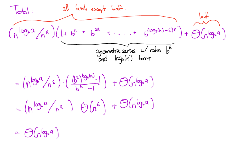
Geometric Series
Before we prove the Master Theorem, let’s review geometric series. A geometric series is a sum that looks like \[ S = a + ar + ar^2 + ... ar^{n-1} = \sum_{i=0}^{n-1} ar^i \]
I.e. each term in the sum is obtained by multiplying the previous term by \(r\).
The closed-form solution for \(S\) is
\[ S = a\left(\frac{r^n - 1}{r - 1}\right) \]
Proof
\(S = a + ar + ar^2 + ... ar^{n-1}\)
Solution
A short proof. \(rS = ar + ar^2 + ... ar^n = S + ar^n - a\). Rearrange.Balanced case
\(f(n) = \Theta(n^{\log_b(a)})\)
\(f(n) = \Theta(n^{\log_b(a)})\)
\(f(n) = \Theta(n^{\log_b(a)})\)
Leaf heavy case
\(f(n) = O(n^{\log_b(a) - \epsilon})\)
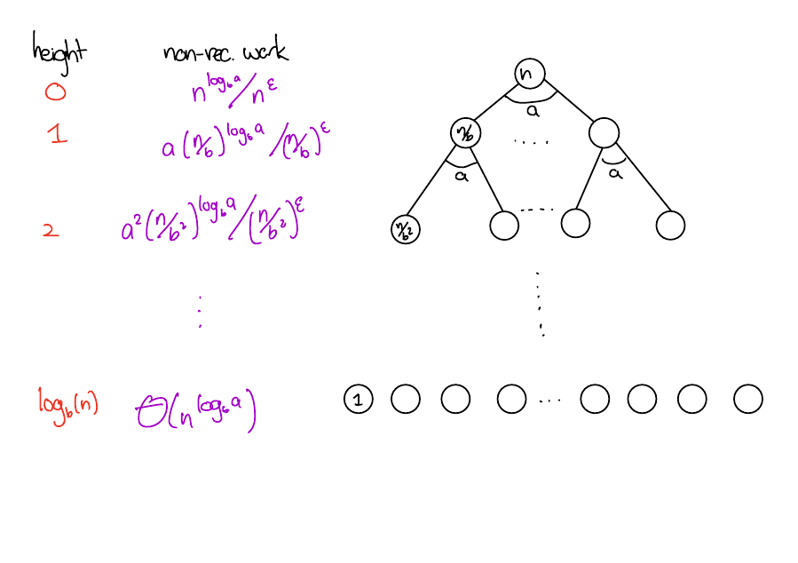
\(f(n) = O(n^{\log_b(a) - \epsilon})\)
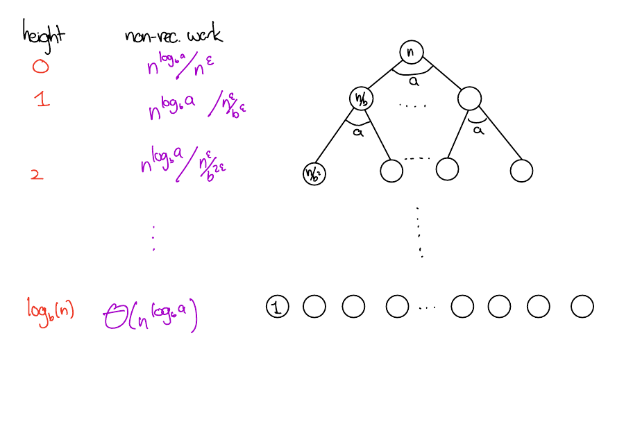
\(f(n) = O(n^{\log_b(a) - \epsilon})\)
Root heavy case
The third case is similar to the previous cases. Check CLRS section 4.6.1 for the details.