7 Evaluation of Yeti

In this chapter we evaluate Yeti from three main perspectives. First, we evaluate the effectiveness of traces for capturing the execution of regions of Java programs, and verify that the frequency of dispatching region bodies does not burden overall performance. Second, we confirm that the performance of the simplest, entry level, version of our system is reasonable, and that performance improves as more sophisticated shapes of region bodies are identified and effort is invested in compiling them. The goal here is to determine whether the first few stages of our extensible system are viable deployment candidates for an incrementally evolving system. Third, we attempt to measure the extent to which our technique is affected by various pipeline hazards, especially branch mispredictions and instruction cache misses.

We prototyped Yeti in a Java VM (rather than a language that does not have a JIT) in order to compare our techniques against high-quality implementations on well-known benchmarks. We show that through four stages of extending our system, from a simple direct call-threaded (DCT) interpreter to a trace based JIT compiler, performance improves steadily. Moreover, at each stage, the performance of our system is comparable to other Java implementations based on different, more specific techniques. Thus, DCT, the entry level of Yeti, is roughly comparable to switch threading. Interpreted traces are faster that direct threading and our trace based JIT is 27 % faster than selective inlining in SableVM.

These results indicate that our design for Yeti is a good starting point for an extensible infrastructure whose performance can be incrementally improved, in contrast to techniques like those described in Chapters  and which are end points with little infrastructure to support the next step up in performance.

sec:YetiEval-Virtual-Machines-Platforms describes the experimental set-up. We report the extent to which different shapes of region enable execution to stay within the code cache in sec:effect-region-shape-dispatchcount. sec:effect-region-shape reports how the performance of Yeti is affected by different region shapes. sec:Early-Pentium-Results describes preliminary performance results on the Pentium. Finally, sec:gpul studies the effect of various pipeline hazards on performance.

1 Experimental Set-up

The experiments described in this section are simpler than those described in cha:Evaluation-of-efficient because we have modified only one Java virtual machine, JamVM. Almost all our performance measurements are made on the same PowerPC machine, except for a preliminary look at interpreted traces on Pentium.

We took a different tack to investigating the micro-architectural impact of our techniques than the approach presented in Chapter . There, we measured specific performance monitoring counters, for instance, the number of mispredicted taken branches that occurred during the execution of a benchmark. Here, we evaluate Yeti's impact on the pipelines using a much more sophisticated infrastructure which determines the causes of various stall cycles.

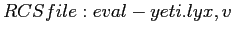
Table: SPECjvm98 benchmarks including elapsed time for baseline JamVM (i.e., without any of our modifications), Yeti and Sun HotSpot.

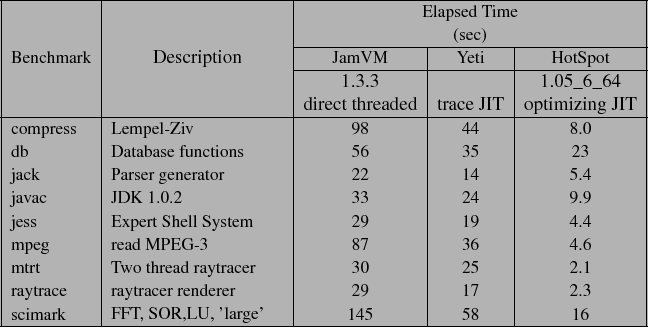
Table: Guide to labels which appear on figures and references to technique descriptions.

1 Virtual Machines

Yeti is a modified version of Robert Lougher's JamVM 1.1.3, which is a very neatly written Java Virtual Machine [#!lougher:jamvmsite!#]. On all platforms (OSX 10.4, PowerPC and Pentium Linux) we built both our modifications to JamVM and JamVM as distributed using gcc 4.0.1.

We compare the performance of Yeti to several other JVM configurations:

1. JamVM configured for direct threading (its default configuration) is our baseline because direct threading is a commonly deployed high performance dispatch technique.
2. JamVM configured to be switch threaded as an example of an entry-level interpretation technique. Many production language virtual machines have been usefully deployed using switch threading.
3. A subroutine threaded version of JamVM.
4. SableVM with selective inlining as an example of an advanced interpreter technique.
5. Sun's Hotspot JVM version 1.05 as a state of the art Java JIT.

2 Elapsed Time Data

Elapsed time performance data was collected on a dual CPU 2 GHz PowerPC 970 processor with 512 MB of memory running Apple OSX 10.4. Pentium performance was measured on a Intel Core 2 Duo E6600 2.40GHz 4M with 2GB of memory under Linux 2.6.9. Performance is reported as the average of three measurements of elapsed time, as printed by the time command.

3 Benchmarks

Table  briefly describes each SPECjvm98 benchmark [#!SPECjvm98!#] and scimark, a scientific program. Since the rest of the figures in this chapter will report performance relative to unmodified JamVM 1.1.3, Table includes, for each benchmark, the raw elapsed time for JamVM, Yeti (running our JIT), and version 1.05.0_6_64 of Sun Microsystems' Java HotSpot JIT. (We provide the elapsed time here because below we will report performance relative to direct threaded JamVM.)

Table  provides a key to the acronyms used as labels in the following graphs and indicates the section of this thesis each technique is discussed.

Pipeline Hazards

In Section  we describe how Yeti is effected by common processor pipeline hazards, such as branch mispredictions and instruction cache misses. We use a new infrastructure, built and operated by Azimi et al., colleagues from the Electrical Engineering Computer Group, that heuristically attributes stall cycles to various causes [#!azimi-ics05!#]. Livio Soares provided us with a port of their infrastructure to Linux 2.6.18. We collected the stall data on a slightly different model of PowerPC, a 2.3 GHz PowerPC 970FX (Apple G5 Xserve) running Linux version 2.6.18. The 970FX part is a 90nm implementation of the 130nm 970, more power efficient but identical architecturally. The platform change was forced upon us because Soares' port requires a system running the new FX version of the processor.

2 Effect of region shape on dispatch

Figure: Number of dispatches executed vs region shape. The y-axis has a logarithmic scale. Numbers above bars, in scientific notation, give the number of regions dispatched. The X axis lists the SPECjvm98 benchmarks in alphabetical order.

Figure: Number of virtual instructions executed per dispatch for each region shape. The y-axis has a logarithmic scale. Numbers above bars are the number of virtual instructions executed per dispatch (rounded to two significant figures). SPECjvm98 benchmarks appear along X axis sorted by the average number of instructions executed by a LB.

In this section we report data obtained by modifying Yeti's instrumentation to keep track of how many virtual instructions are executed from each region body and how often region bodies are dispatched. These data will help us understand to what extent execution remains in the code cache for differently shaped regions of the program.

For a JIT to be effective, execution must spend most of its time in compiled code. We can easily count how many virtual instructions are executed from interpreted traces and so we can calculate what proportion of all virtual instructions executed come from traces. For jack, traces account for 99.3% of virtual instructions executed. For all the remaining benchmarks, traces account for 99.9% or more.

A remaining concern is how often execution enters and leaves the code cache. In our system, execution enters the code cache whenever a region body is called from a dispatch loop. It is an easy matter to instrument the dispatch loops to count how many iterations occur, and hence how many dispatches are made. These numbers are reported by Figure . The figure shows how direct call threading (DCT) compares to linear blocks (LB), interpreted traces with no linking (i-TR-nolink) and linked interpreted traces (i-TR). Note that the y-axis has a logarithmic scale.

DCT dispatches each virtual instruction body individually, so the DCT bars on Figure  report how many virtual instructions were executed by each benchmark. For each benchmark, the ratio of DCT to LB shows the dynamic average linear block length (e.g., for compress the average linear block executed virtual instructions). In general, the height of each bar on Figure  divided by the height of the DCT bar gives the average number of virtual instructions executed per dispatch of that region shape. Figure  also presents the same data in terms of virtual instructions executed per dispatch, but sorts the benchmarks along the x axis by the average LB length. Hence, for compress, the LB bar shows 9.9 virtual instructions executed on the average.

Scientific benchmarks appear on the right of Figure  because they tend to have longer linear blocks. For instance, the average block in scitest has about 24 virtual instructions whereas javac, jess and jack average about 4 instructions. Comparing the geometric mean across benchmarks, we see that LB reduces the number of dispatches relative to DCT by a factor of 6.3. On long basic block benchmarks, we expect that the performance of LB will approach that of direct threading for two reasons. First, fewer trips around the dispatch loop are required. Second, we showed in Chapter  that subroutine threading is better than direct threading for linear regions of code.

Traces do predict paths taken through the program. The rightmost cluster on Figure  show that, even without trace linking (i-TR-nolink), the average trace executes about 5.7 times more virtual instructions per dispatch than a LB. The improvement can be dramatic. For instance javac executes, on average, about 22 virtual instructions per trace dispatch. This is much longer than its dynamic average linear block length of 4 virtual instructions. This means that for javac, on the average, the fourth or fifth trace exit is taken. Or, putting it another way, for javac a trace typically correctly predicts the destination of 5 or 6 virtual branches.

This behavior confirms the assumptions behind our approach to handling virtual branch instructions in general and the design of interpreted trace exits in particular. We expect that most of the trace exits, four fifths in the case of javac, will not exit. Hence, we generate code for interpreted trace exits that should be easily predicted by the processor's branch history predictors. In the next section we will show that this improves performance, and in Section  we show that it also reduces branch mispredictions.

Adding trace linking completes the interpreted trace (i-TR) technique. Trace linking makes the greatest single contribution, reducing the number of times execution leaves the trace cache by between one and 3.7 orders of magnitude. Trace linking has so much impact because it links traces together around loops. A detailed discussion of how inner loops depend on trace linking appears in Section .

Figure: Percentage trace completion rate as a proportion of the virtual instructions in a trace and code cache size for as a percentage of the virtual instructions in all loaded methods. For the SPECjvm98 benchmarks and scitest.

Although this data shows that execution is overwhelmingly from the trace cache, it gives no indication of how effectively code cache memory is being used by the traces. A thorough treatment of this, like the one done by Bruening and Duesterwald [#!UnitShapes00!#], is beyond the scope of this thesis. Nevertheless, we can relate a few anecdotes based on data that our profiling system already collects.

Figure  describes two aspects of traces. First, in the figure, the %complete bars report the extent to which traces typically complete, measured as a percentage of the virtual instructions in a trace. For instance, for raytrace, the average trace exit occurs after executing 59% of the virtual instructions in the trace. Second, the %loaded bars report the size of the traces in the code cache as a percentage of the virtual instructions in all the loaded methods. For raytrace we see that the traces contain, in total, 131% of the code in the underlying loaded methods. Closer examination of the trace cache shows that raytrace contains a few very long traces which reach the 100 block limit (See Section ). In fact, there are nine such traces generated for raytrace, one of which is dispatched 500 thousand times. (This is the only 100 block long trace executed more than a few thousand times generated by any of our benchmarks.) The hot trace was generated from code performing a complex calculation with many calls to small accessor methods that were inlined into the trace, hence the high block count. Interestingly, this trace has several hot trace exits, the last significantly hot exit from the 68'th block.

We observe that for an entire run of the scitest benchmark, all generated traces contain only 24% of the virtual instructions contained in all loaded methods. This is a good result for traces, suggesting that a trace-based JIT needs to compile fewer virtual instructions than a method-based JIT. Also, we see that for scitest, the average trace executes almost to completion, exiting after executing 99% of the virtual instructions in the trace. This is what one would expect for a program that is dominated by inner loops with no conditional branches - the typical trace will execute until the reverse branch at its end.

On the other hand, for javac we find the reverse, namely that the traces bloat the code cache - almost four times as many virtual instructions appear in traces than are contained in the loaded methods. In Section  we shall discuss the impact of this on the instruction cache. Nevertheless, traces in javac are completing only modestly less than the other benchmarks. This suggests that javac has many more hot paths than the other benchmarks. What we are not in a position to measure at this point is the temporal distribution of the execution of the hot paths.

3 Effect of region shape on performance

In this section we report the elapsed time required to execute each benchmark. One of our main goals is to create an architecture for a high level machine that can be gradually extended from a simple interpreter to a high performance JIT augmented system. Here, we evaluate the performance of various stages of Yeti's enhancement from a direct call-threaded interpreter to a trace based mixed-mode system.

Figure: Performance of each stage of Yeti enhancement from DCT interpreter to trace-based JIT relative to unmodified JamVM-1.3.3 (direct-threaded) running the SPECjvm98 benchmarks (sorted by LB length).

Figure  shows how performance varies as differently shaped regions of the virtual program are executed. The figure shows elapsed time relative to the unmodified JamVM distribution, which uses direct-threaded dispatch. The raw performance of unmodified JamVM and TR-JIT is given in Table . The first four bars in each cluster represent the same stage of Yeti's enhancement as those in Figure . The fifth bar, TR-JIT, gives the performance of Yeti with our JIT enabled.

1 Direct Call Threading

Our simplest technique, direct call threading (DCT) is slower than JamVM, as distributed, by about 50%.

Although this seems serious, we note that many production interpreters are not direct threaded but rather use the slower and simpler switch threading technique. When JamVM is configured to run switch threading we we find that its performance is within 1% of DCT. This suggests that the performance of DCT is well within the useful range.

2 Linear Blocks

Figure: Performance of Linear Blocks (LB) compared to subroutine-threaded JamVM-1.3.3 (SUB) relative to unmodified JamVM-1.3.3 (direct-threaded) for the SPECjvm98 benchmarks.

As can be seen on Figure , Linear blocks (LB) run roughly 30% faster than DCT, matching the performance of direct threading for benchmarks with long basic blocks like compress and mpeg. On the average, LB runs only 15% more slowly than direct threading.

The region bodies identified at run time by LB are very similar to the code generated by subroutine threading (SUB) at load time so one might expect the performance of the two techniques to be the same. However, as shown by Figure  LB is, on the average, about 43% slower.

This is because virtual branches are much more expensive for LB. In SUB, the virtual branch body is called from the CTT, then, instead of returning, it executes an indirect branch directly to the destination CTT slot. In contrast, in LB a virtual branch instruction sets the vPC and returns to the dispatch loop to call the destination region body. In addition, each iteration of the dispatch loop must loop up the destination body in the dispatcher structure (through an extra level of indirection compared to SUB).

3 Interpreted Traces

Figure: Performance of JamVM interpreted traces (i-TR) and selective inlined SableVM 1.1.8 relative to unmodified JamVM-1.3.3 (direct-threaded) for the SPECjvm98 benchmarks.

Figure: Performance of JamVM interpreted traces (i-TR) relative to unmodified JamVM-1.3.3 (direct-threaded) and selective inlined SableVM 1.1.8 relative to direct threaded SableVM version 1.1.8 for the SPECjvm98 benchmarks.

Just as LB reduces dispatch and performs better than DCT, so link-disabled interpreted traces (i-TR-nolink) further reduce dispatch and run 38% faster than LB.

Interpreted traces implement virtual branch instructions better than LB or SUB. As described in Section , i-TR generates a trace exit for each virtual branch. The trace exit is implemented as a direct conditional branch that is not taken when execution stays on trace. As we have seen in the previous section, execution typically remains on trace for several trace exits. Thus, on the average, i-TR replaces costly indirect calls (from the dispatch loop) with relatively cheap not-taken direct conditional branches. Furthermore, the conditional branches are fully exposed to the branch history prediction facilities of the processor.

Trace linking, though it eliminates many more dispatches, achieves only a modest further speed up because the specialized dispatch loop for traces is much less costly than the generic dispatch loop that runs LB.

We compare the performance of selective inlining, as implemented by SableVM, and interpreted traces in two different ways. First, in Figure , we compare the performance of both techniques relative to the same baseline, in this case JamVM with direct threading. Second, in Figure , we show the speedup of each VM relative to its own implementation of direct threading, that is, we show the speedup of i-TR relative to JamVM direct threading and selective inlining relative to SableVM direct threading.

Overall, Figure  shows that i-TR and SableVM perform almost the same with i-TR about 3% faster than selective inlining. SableVM wins on programs with long basic blocks, like mpeg and scitest, because selective inlining eliminates dispatch from long sequences of simple virtual instructions. However, i-TR wins on shorter block programs like javac and jess by improving branch prediction. Nevertheless, Figure  shows that selective inlining results in a 2% larger speedup over direct threading for SableVM than i-TR. Both techniques result in very similar overall effects even though i-TR is focused on improving virtual branch performance and selective inlining on eliminating dispatch within basic blocks.

Subroutine threading again emerges as a very effective interpretation technique, especially given its simplicity. SUB runs only 6% more slowly than i-TR and SableVM.

The fact that i-TR runs exactly the same runtime profiling instrumentation as TR-JIT makes it qualitatively a very different system than SUB or SableVM. SUB and SableVM are both tuned interpreters that generate a small amount of code at load time to optimize dispatch. Neither includes any profiling infrastructure. In contrast to this, i-TR runs all the infrastructure needed to identify hot traces at run time. As we shall see in Section , the improved virtual branch performance of interpreted traces has made it possible to build a profiling system that runs faster than most interpreters.

4 JIT Compiled traces

Figure: Elapsed time performance of Yeti with JIT compared to Sun Java 1.05.0_6_64 relative to JamVM-1.3.3 (direct threading) running SPECjvm98 benchmarks.

The rightmost bar in each cluster of Figure shows the performance of our best-performing version of Yeti (TR-JIT). Comparing geometric means, we see that TR-JIT is roughly 24% faster than interpreted traces. Despite supporting only 50 integer and object virtual instructions, our trace JIT improves the performance of integer programs such as compress significantly. With our most ambitious optimization, of virtual method invocation, TR-JIT improved the performance of raytrace by about 35% over i-TR. Raytrace is written in an object-oriented style with many small methods invoked to access object fields. Hence, even though it is a floating-point benchmark, it is greatly improved by devirtualizing and inlining these accessor methods.

Figure compares the performance of TR-JIT to Sun Microsystems' Java HotSpot JIT. Our current JIT runs the SPECjvm98 benchmarks 4.3 times slower than HotSpot. Results range from 1.5 times slower for db, to 12 times slower for mtrt. Not surprisingly, we do worse on floating-point intensive benchmarks since we do not yet compile the float bytecodes.

4 Early Pentium Results

As illustrated earlier, in Figure , the Intel's Pentium architecture takes a different approach to indirect branches and calls than does the PowerPC. On the PowerPC, we have shown that the two-part indirect call used in Yeti's dispatch loops performs well. However, the Pentium relies on its BTB to predict the destination of its indirect call instruction. As we saw in Chapter , when the prediction is wrong, many stall cycles may result. Conceivably, on the Pentium, the unpredictability of the dispatch loop indirect call could lead to very poor performance.

Gennady Pekhimenko, a fellow graduate student at the University of Toronto, ported i-TR to the Pentium platform. Figure  gives the performance of his prototype. The results are roughly comparable to our PowerPC results, though i-TR outperforms direct threading a little less on the Pentium. The average test case ran in 83% of the time taken by direct threading whereas it needed 75% on the PowerPC.

Figure: Performance of Gennady Pekhimenko's Pentium port relative to unmodified JamVM-1.3.3 (direct-threaded) running the SPECjvm98 benchmarks.

5 Identification of Stall Cycles

We have shown that Yeti performs well compared to existing interpreter techniques. However, much of our design is motivated by micro-architectural considerations. In this section, we use a new set of tools to measure the stall cycles experienced by Yeti as it runs.

The purpose of this analysis is twofold. First, we would like to confirm that we understand why Yeti performs well. Second, we would like to discover any source of stalls we did not anticipate, and perhaps find some guidance on how we could do better.

1 Identifying Causes of Stall Cycles

Azimi et al. [#!azimi-ics05!#] describe a system that uses a statistical heuristic to attribute stall cycles in a PowerPC 970 processor. They define a stall cycle as a cycle for which there is no instruction that can be completed. Practically speaking, on a PowerPC970, this occurs when the processor's completion queue is empty because instructions are held up, or stalled. Their approach, implemented for a PPC970 processor running K42, a research operating system [#!k42:website!#], exploits performance monitoring hardware in the PowerPC that recognizes when the processor's instruction completion queue is empty. Then, the next time an instruction does complete they attribute, heuristically and imperfectly, all the intervening stall cycles to the functional unit of the completed instruction. Azimi et al. show statistically that their heuristic estimates the true causes of stall cycles well.

The Linux port runs only on a PowerPC 970FX processor. This is slightly different than the PowerPC 970 processor we have been using up to this point. The only acceptable machine we have access to is an Apple Xserve system which was also slightly faster than our machine, running at 2.3 GHz rather than 2.0 GHz.

Table: GPUL categories

2 Stall Cycle results

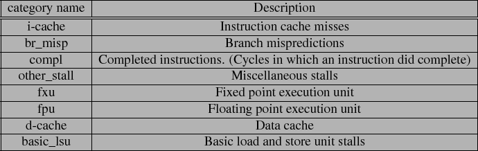
Figure: Cycles relative to JamVM-1.3.3 (direct threading) running SPECjvm98 benchmarks.

Figure  shows the break down of stall cycles for various runs of the SPECjvm98 benchmarks as measured by the tools of Azimi et al. Five bars appear for each benchmark. From the left to the right, the stacked bars represent subroutine-threaded JamVM 1.1.3 (SUB) , JamVM 1.1.3 (direct-threaded as distributed, hence DISTRO) and three configurations of Yeti, i-TR-no-link, i-TR and TR-JIT. The y axis, like many of our performance graphs, reports performance relative to JamVM. The height of the DISTRO bar is thus 1.0 by definition. Figure  reports the same data as Figure , but, in order to facilitate pointing out specific trends, zooms in on four specific benchmarks.

Each histogram column is split vertically into a stack of bars which illustrates how executed cycles break down by category. Only cycles listed as ``compl'' represent cycles in which an instruction completed. All the other categories represent stalls, or cycles in which the processor was unable to complete an instruction. The ``other_stall'' category represents stalls to which the tool was not able to attribute a cause. Unfortunately, the other_stall category includes a source of stalls that is important to our discussion, namely the stalls caused by data dependency between the two instructions of the PowerPC architectures' two-part indirect branch mechanism. See Figure  for an illustration of two-part branches.

Figure: Stall breakdown for SPECjvm98 benchmarks relative to JamVM-1.3.3 (direct threading).

The total cycles executed by each benchmark do not correlate perfectly with the elapsed time measurements reported earlier in this chapter.

For instance, in Figure , i-TR runs scitest in 60% of the time of direct threading, whereas in Figure (c) it takes 80%. There are a few important differences between the runs, namely the differences between the PowerPC 970FX and PowerPC 970, the different clock speed (2.3 GHz vs 2.0 GHz) and differences between Linux (with modifications made by Azimi et al.) and OSX 10.4. We use the data qualitatively to characterize pipeline hazards and not to measure absolute performance.

3 Trends

Several interesting trends emerge from our examination of the cycle reports.

1. Interpreted traces reduce branch mispredictions caused by virtual branch instructions.
2. Simple code we generated for interpreted trace exits stresses the fixed-point execution unit (fxu)
3. Our JIT (TR-JIT) does little to reduce lsu stalls, which is a surprise since many loads and stores to the expression stack are eliminated by the register allocator.
4. As we reduce pipeline hazards caused by dispatch new kinds of stalls arise.
5. Trace bloat, like we observed for javac, can lead to significant stalls due to instruction cache misses.

Each of these issues will be discussed in turn.

1 Branch misprediction

In Figure (mpeg) we see how our techniques affect mpeg, which has a few very hot, very long basic blocks. The blocks contain many duplicate virtual instructions. Hence, direct threading encounters difficulty due to the context problem, as discussed in Section . (This is plainly evident in the solid red br_misp stack on the DISTRO bar on all four sub figures.)

SUB reduces the mispredictions that occur running mpeg significantly - presumably the ones caused by linear regions. Yeti's i-TR technique effectively eliminates the branch mispredictions for mpeg altogether. Both techniques also reduce other_stall cycles relative to direct threading. These are probably being caused by the PowerPC's two-part indirect branches which are used by DISTRO to dispatch all virtual instructions and by SUB to dispatch virtual branches. SUB eliminates the delays for straight-line code and i-TR further eliminates the stalls for virtual branches. Figures (javac) and (jess) show that traces cannot predict all branches and some stalls due to branch mispredictions remain for i-TR and TR-JIT.

2 Overhead of interpreted Trace Exits

In all four sub figures of Figure  we see that fxu stalls decrease or stay the same relative to DISTRO for SUB whereas for i-TR they increase. Note also that the fxu stalls decrease again for the TR-JIT condition. This suggests that the fxu stalls are not caused by the overhead of profiling (since TR-JIT runs exactly the same instrumentation as i-TR). Rather, they are caused by the overhead of the simple-minded trace exit code we generate for interpreted traces.

Recall that interpreted traces generate a compare immediate of the vPC followed by a conditional branch. The comparand is the destination vPC, a 32 bit number. On a PowerPC, there is no form of the compare immediate instruction that takes a 32 bit immediate parameter. Thus, we generate two fixed point load immediate instructions to load the immediate argument into a register. Presumably it is these fixed point instructions that are causing the extra stalls.

3 TR-JIT and the Expression Stack

Yeti's compiler works hard to eliminate loads and stores to and from Java's expression stack. In Figure (mpeg) , TR-JIT makes a large improvement over i-TR by reducing the number of completed instructions. However, it was surprising to learn that basic_lsu stalls were in fact not much effected. (This pattern holds across all the other sub figures also.) Presumably the pops from the expression stack hit the matching pushes in PPC970's store pending queue and hence were not stalling in the first place.

4 Exposing stalls from workload

In Figure (scitest) we see an increase in stalls due to the FPU for SUB and i-TR. Our infrastructure makes no use of the FPU at all - so presumably this happens because stalls waiting on the real work of the application are exposed as we eliminate other pipeline hazards.

This effect makes it hard to draw conclusions about any increase in stalls that occurs, for instance the increase in fxu stalls caused by i-TR described in the previous section, because it might also be caused by the application.

5 Trace bloat

The javac compiler is a big benchmark. The growth of the blue hatched bars at the top of Figure (javac) shows how i-TR and TR-JIT make this significantly worse. Even SUB, which only generates one additional 4 byte call per virtual instruction, increases i-cache misses. In the figure, i-TR stalls on instruction cache as much as direct threading stalls on mispredicted branches.

As we pointed out in Section , Dynamo's trace selection heuristic does not work well for javac, selecting traces representing four times as many virtual instructions as appear in all the loaded methods. This happens when many long but slightly different paths are hot through a body of code. Part of the problem is that the probability of reaching the end of a long trace under these conditions is very low. As trace exits become hot more traces are generated and replicate even more code. As more traces are generated the trace cache grows huge.

Figure (javac) shows that simply setting aside a large trace cache is not a good solution. The replicated code in the traces makes the working set of the program larger than the instruction cache can hold.

Our system does not, at the moment, implement any mechanism for reclaiming memory that has been assigned to a region body. An obvious candidate would be reactive flushing (See Section ), which occasionally flushes the trace cache entirely. This may result in better locality of reference after the traces are regenerated anew. Counter-intuitively, reducing the size of the trace cache and implementing a very simple trace cache flushing heuristic may lead to better instruction cache behavior than setting aside a large trace cache.

Hiniker et al [#!hiniker-trace-select-improvements!#] have suggested several changes to the trace selection heuristic that improve locality and reduce replication between traces.

6 Chapter Summary

We have shown that traces, and especially linked traces, are an effective shape for region bodies. The trace selection heuristic described by the HP Dynamo project, described in Section , results in execution from the code cache for an average or 2000 virtual instructions between dispatches. This reduces the overhead of region body dispatch to a negligible level. The amount of code cache memory required to achieve this seems to vary widely by program, from a very parsimonious 24% of the virtual instructions in the loaded methods for scitest to a rather bloated 380% for javac.

We have measured the performance of four stages in the evolution of Yeti: DCT, LB, i-TR, and TR-JIT. Performance has steadily improved as larger region bodies are identified and translated. Traces have proven to be an effective shape for region bodies for two main reasons. First, interpreted traces offer a simple and efficient way to efficiently dispatch both straight line code and virtual branch instructions. Second, compiling traces is straightforward - in part because the JIT can fall back on our callable virtual instruction bodies, but also because traces contain no merge points, which makes compilation easy.

Interpreted traces are a fast way of interpreting a program, despite the fact that runtime profiling is required to identify traces. We show that interpreted traces are just as fast as inline-threading, SableVM's implementation of selective inlining. Selective inlining eliminates dispatch within basic blocks at runtime (Section ) whereas interpreted traces eliminate branch mispredictions caused by the dispatch of virtual branch instructions. This suggests that a hybrid, namely inlining bodies into interpreted traces (reminiscent of our TINY inlining heuristic of Section ) may be an interesting intermediate technique between interpreted traces and the trace-based JIT.

Yeti provides a design trajectory by which a high level language virtual machine can be extended from a simple interpreter to a sophisticated trace-based JIT compiler mixed-mode virtual machine. Our strategy is based on two key assumptions. First, that stepping back to a relatively slow dispatch technique, direct call threading (DCT), is worthwhile. Second, that identifying dynamic regions of the program at runtime, traces, should be done early in the life of a system because it enables high performance interpretation.

In this chapter we have shown that both these assumptions are reasonable. Our implementation of DCT performs no worse than switch threading, commonly used in production, and the combination of trace profiling and interpreted traces is competitive with high-performance interpreter optimizations. This is in contrast to context threading, selective inlining, and other dispatch optimizations, which perform about the same as interpreted traces but do nothing to facilitate the development of a JIT compiler.

A significant remaining challenge is how best to implement callable virtual instruction bodies. The approach we follow, as illustrated by Figure , is efficient but depends on C language extensions and hides the true control flow of the interpreter from the compiler that builds it. A possible solution to this will be touched upon in Chapter .

The cycle level performance counter infrastructure provided by Azimi et al. has enabled us to learn why our technique does well. As expected, we find that traces make it easier for the branch prediction hardware to do its job, and thus stalls due to branch mispredictions reduce markedly. To be sure, some paths are still hard to predict and traces do not eliminate all mispredicted branches. We find that the extra path length of interpreted trace exits does matter, but in the balance reduces stall cycles from mispredicted branches more than enough to improve performance overall.

Yeti is early in its evolution at this point. Given the robust performance increases we obtained compiling the first 50 integer instructions we believe much more performance can be easily obtained just by compiling more kinds of virtual instructions. For instance, floating point multiplication (FMUL or DMUL) appears amongst the most frequently executed virtual instructions in four benchmarks (scitest, ray, mpeg and mtrt). We expect that our gradual approach will allow these virtual instructions to compiled next with commensurate performance gains.