CSC321 Home Lectures, Readings and Due Dates Optional Readings Tutorials Computing Assignments Tests Anthony Bonner's Homepage: www.cs.toronto.edu/~bonner

CSC321 Spring 2016 – Lectures, Readings and Due Dates The lectures are Wednesday 3-5pm in IB 335. Tentative Schedule: January 6. Lecture 1: [slides] Lecture 1a: Why do we need machine learning? Lecture 1b: What are neural networks? Lecture 1c: Some simple models of neurons Lecture 1d: A simple example of learning Lecture 1e: Three types of learning Lecture 2: [slides] Lecture 2a: Types of neural network architectures Lecture 2b: Perceptrons: The first generation of neural networks January 13. Lecture 2 [continued] Lecture 2c: A geometrical view of perceptrons Lecture 2d: Why the learning works Lecture 2e: What perceptrons can't do Lecture 3: [slides] Lecture 3a: Learning the weights of a linear neuron Lecture 3b: The error surface for a linear neuron Lecture 3c: Learning the weights of a logistic output neuron January 20. Lecture 3 [continued]: Lecture 3d: The backpropagation algorithm [reading] Lecture 3e: Using the derivatives computed by backpropagation Lecture 4: [slides] Lecture 4a: Learning to predict the next word Lecture 4b: A brief diversion into cognitive science Lecture 4c: Another diversion: The softmax output function Written material: The math of softmax units Lecture 4d: Neuro-probabilistic language models [reading] January 27. 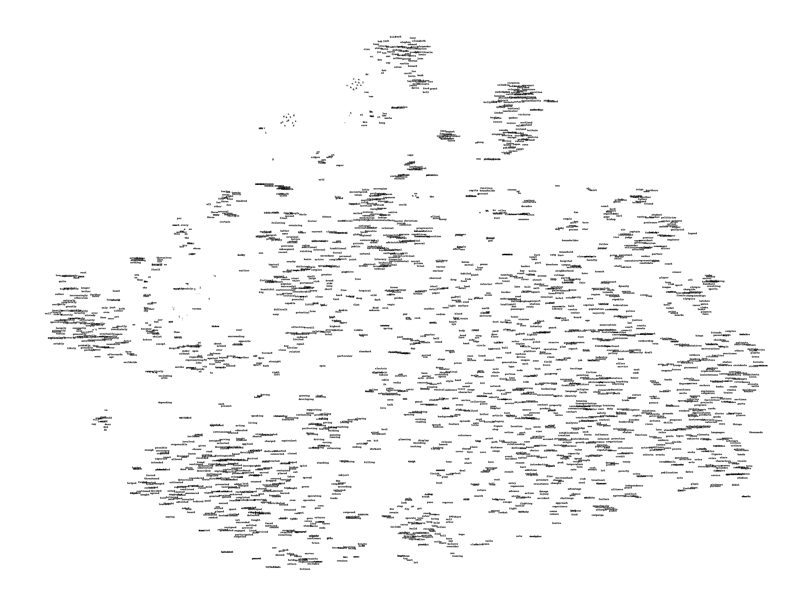Lecture 4 [continued]: Lecture 4e: Ways to deal with the large number of possible outputs [word map] Lecture on distributed representations and coarse coding [slides]. Lecture 5: [slides] Lecture 5a: Why object recognition is difficult Lecture 5b: Achieving viewpoint invariance Lecture 5c: Convolutional nets for digit recognition Lecture 5d: Convolutional nets for object recognition [reading1] [reading2] January 28.  Assignment 1 is posted. February 3. Lecture 6: [slides] Lecture 6a: Overview of mini-batch gradient descent Lecture 6b: A bag of tricks for mini-batch gradient descent Lecture 6c: The momentum method Lecture 6d: Adaptive learning rates for each connection Lecture 6e: Rmsprop: Divide the gradient by a running average of its recent magnitude February 4.  Assignment 1 is due. February 10. Lecture 9: [slides] Lecture 9a: Overview of ways to improve generalization Lecture 9b: Limiting the size of the weights Lecture 9c: Using noise as a regularizer Lecture 9d: Introduction to the full Bayesian approach Lecture 9e: The Bayesian interpretation of weight decay Lecture 10: [slides] Lecture 10a: Why it helps to combine models Lecture 10b: Mixtures of Experts [reading] February 11.  Assignment 2 is posted. February 17: No Lecture (reading week) February 24. Lecture 10 [continued] Lecture 10c: The idea of full Bayesian learning Lecture 10d: Making full Bayesian learning practical Lecture 10e: Dropout [reading] Lecture on clustering and mixtures of Gaussians [slides] February 25.  Assignment 2 is due. February 26.  Midterm test (in tutorial, starting at 1:10pm sharp) March 2. Review of Lecture 2a. Lecture 7: [slides] Lecture 7a: Modeling sequences: A brief overview Lecture 7b: Training RNNs with back propagation Lecture 7c: A toy example of training an RNN Lecture 7d: Why it is difficult to train an RNN Lecture 7e: Long-term Short-term-memory [movie] [reading] March 3.  Assignment 3 is posted March 9. Lecture 11: [slides] Lecture 11a: Hopfield nets Lecture 11b: Dealing with spurious minima Lecture 11c: Hopfield nets with hidden units Lecture 11d: Using stochastic units to improve search Lecture 11e: How a Boltzmann machine models data [reading] Lecture 12: [slides] Lecture 12a: Boltzmann machine learning March 10.  Assignment 3 is due. March 16. Review of Hopfield nets and Boltzmann machines Lecture 12 [continued] Lecture 12c: Restricted Boltmann Machines Lecture 12d: An example of RBM learning March 23: Lecture 14 [slides] Lecture 14a: Learning layers of features by stacking RBMs [movie] Lecture 14b: Discriminative learning for Deep Belief Nets Lecture 14c: What happens during discriminative fine-tuning? Lecture 14d: Modelling real-valued data with an RBM March 24: Assignment 4 is posted. March 30. Review of Lectures 14a,b,c Lecture 15: [slides] Lecture 15a: From PCA to autoencoders Lecture 15b: Deep autoencoders April 1: Assignment 4 is due.