Introduction
TensorFlow™ is an open source machine learning library for Python (and C++) initially developed by the Google Brain Team for research and released under the Apache 2.0 Open Source License on November 9th, 2015 . It is currently used by Google in their speech recognition, Gmail, Google Photos, Search services and recently adopted by the DeepMind team .
Features
Though TensorFlow was built with deep learning in mind, its framework is general enough so that we can also implement clustering methods, graphical models, optimization problems and others. It also features automatic differentiation, which means that gradients are calculated automatically and therefore backpropagation doesn’t have to be coded by hand (this may not look like much considering the gradients we have seen in linear regression but they get considerably more complex as we approach deep, convolutional or recurrent neural networks). It also performs automatic parallelization and deployment to GPU through CUDA, which is a mandatory feature for any machine learning framework considering the performance edge that GPUs have over CPUs in the field .
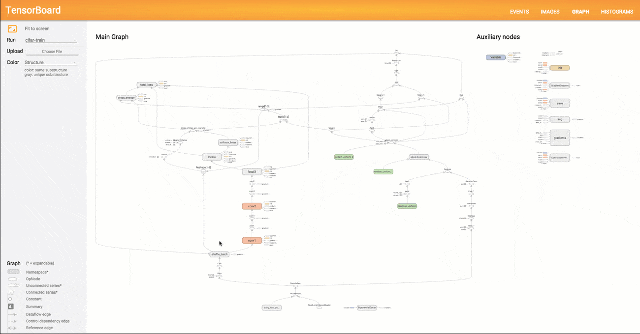
Another nice feature of TensorFlow is TensorBoard, which is a tool that allows us to visualize our computation graph (effectively converting our model code to a graphical representation), keep track of model performance and how our parameters are behaving, among other features.
From now on we will be mostly using TensorFlow to code our models so we will discuss other features as they become meaningful to us.
Special Consideration
TensorFlow essentialy works by defining a data flow graph, where edges represent the data and nodes, the operations. So note that unlike NumPy, in TensorFlow you define a computation graph using tensors, therefore if you have tensors w, x and b, making wx+b won’t actually compute the result right away, but rather add a node on the computation graph that corresponds to this operation, the numerical results will only be calculated once you deploy the model to the CPU/GPU. The concept might feel strange at first if you’re not used to this paradigm but it becomes natural after a while and has the added advantage of increasing performance.
Installation
To install TensorFlow follow the continuously updated official guide available in https://www.tensorflow.org/get_started. If you have a compatible NVIDIA card make sure to install the GPU-Enabled version. Also, I would personally recommend that you install TensorFlow using a conda environment, but simply using pip will work as well.
If you run into any problems during the installation, feel free to leave a comment below or contact me.
Linear Regression in TensorFlow
To briefly illustrate how TensorFlow works we’ll be reimplementing the model from our last tutorial on Multiple Linear Regression. We use the same initial setup, except we’ll be changing our data to promote some diversity.
import numpy as np
import matplotlib.pyplot as plt
import tensorflow as tf

# NEW DATA
data_x = np.linspace(1, 8, 100)[:, np.newaxis]
data_y = np.polyval([1, -14, 59, -70], data_x) \
        + 1.5 * np.sin(data_x) + np.random.randn(100, 1)
# --------

model_order = 5
data_x = np.power(data_x, range(model_order))
data_x /= np.max(data_x, axis=0)

order = np.random.permutation(len(data_x))
portion = 20
test_x = data_x[order[:portion]]
test_y = data_y[order[:portion]]
train_x = data_x[order[portion:]]
train_y = data_y[order[portion:]]
We now proceed to define our computation graph or, in other words, define our model. We start by defining our input and correct output placeholders, which act as, well, placeholders for our training data. We first determine its type (float32), shape (where you can use a single “None” in it to have an unrestricted dimension, allowing us to feed sequences or batches of different lengths) and a name, which will be used by TensorBoard.
with tf.name_scope("IO"):
    inputs = tf.placeholder(tf.float32, [None, model_order], name="X")
    outputs = tf.placeholder(tf.float32, [None, 1], name="Yhat")
Next we define our actual linear regression model, which in our convention is simply a matrix multiplication by the weight parameter. To define our parameters we use Variables, which differ from placeholder in the sense that they are trainable, therefore whenever you add a new variable to your model, unless if stated otherwise, TensorFlow will infer a gradient for it and tune it during training. We then use tf.matmul to compute the matrix multiplication, though just doing *inputsW would work just as well.
with tf.name_scope("LR"):
    W = tf.Variable(tf.zeros([model_order, 1], dtype=tf.float32), name="W")
    y = tf.matmul(inputs, W)
Finally we define our cost function and optimizer. Notice the “trainable=False” flag in the learning_rate variable, that tells TensorFlow not to automatically train this variable. After that we use TF built-in functions to define our mean squared error loss and then we tell it to use Gradient Descent with a learning rate of learning_rate to minimize the cost.
with tf.name_scope("train"):
    learning_rate = tf.Variable(0.5, trainable=False)
    cost_op = tf.reduce_mean(tf.pow(y-outputs, 2))
    train_op = tf.train.GradientDescentOptimizer(learning_rate).minimize(cost_op)
And that is it for the modeling, no need to define gradients or manually updating parameters. We now proceed to deploy the model to the GPU and feed our training data.
tolerance = 1e-3

# Perform Stochastic Gradient Descent
epochs = 1
last_cost = 0
alpha = 0.4
max_epochs = 50000

sess = tf.Session() # Create TensorFlow session
print "Beginning Training"
with sess.as_default():
    init = tf.initialize_all_variables()
    sess.run(init)
    sess.run(tf.assign(learning_rate, alpha))
    while True:
        # Execute Gradient Descent
        sess.run(train_op, feed_dict={inputs: train_x, outputs: train_y})

        # Keep track of our performance
        if epochs%100==0:
            cost = sess.run(cost_op, feed_dict={inputs: train_x, outputs: train_y})
            print "Epoch: %d - Error: %.4f" %(epochs, cost)

            # Stopping Condition
            if abs(last_cost - cost) < tolerance or epochs > max_epochs:
                print "Converged."
                break
            last_cost = cost

        epochs += 1

    w = W.eval()
    print "w =", w
    print "Test Cost =", sess.run(cost_op, feed_dict={inputs: test_x, outputs: test_y})
We must first create a Session with tf.Session(), which automatically binds to the GPU or CPU, acording to availability or user settings. After setting an environment with our newly created session we initialize our variables (remember that up until now they were just tensors, no actual numerical values associated) and proceed to our training loop.
Lets take a closer look at the sess.run() function. We can call it over any previously defined tensor, if it is an operation (y and train_op, the nodes in our graph) we must also provide the values for all the necessary placeholders, so in sess.run(cost_op, feed_dict={inputs: train_x, outputs: train_y}) we’re telling TensorFlow to execute a gradient descent step using train_x as the input value and train_y as the expected output. Notice that if we wanted just the model output, and not to actually train it, we could simply do sess.run(y, feed_dict={inputs: train_x}) since the model prediction does not depend on the correct answer.
On the other hand, if we call sess.run() on a variable it will simply return its current value. So doing sess.run(var) is equivalent to var.eval().
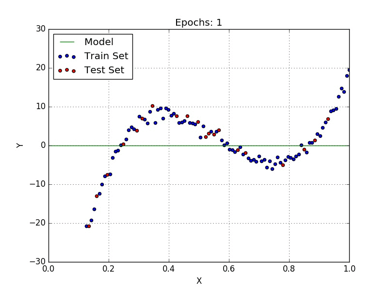
Now we can just run the code and it will automatically train our model until the stopping criteria is satisfied, as can be seen in Fig. 2.
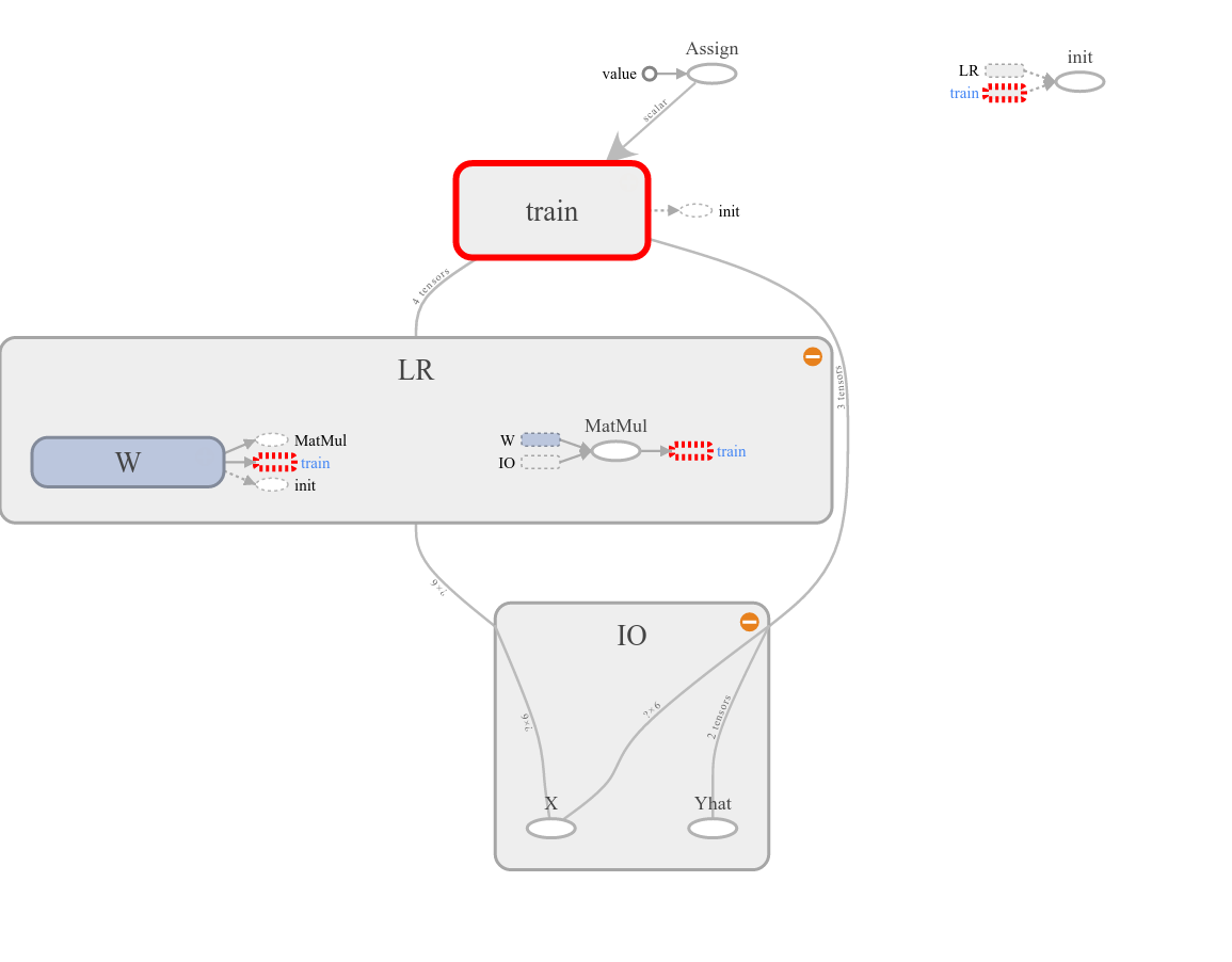
Visualizing our model in TensorBoard yields Fig. 3.
In the next article we will start talking about classification problems and introduce the k-Nearest Neighbors method and Logistic Regression, which puts us just one step away from actually using neural networks.
Jupyter notebook available here
Last modified: June 1, 2016 comments powered by Disqus