This post is a continuation of Linear Regression.
Introduction
In multiple linear regression we extend the notion developed in linear regression to use multiple descriptive values in order to estimate the dependent variable, which effectively allows us to write more complex functions such as higher order polynomials ($y = \sum_{i_0}^{k} w_ix^i$), sinusoids ($y = w_1 sin(x) + w_2 cos(x)$) or a mix of functions ($y = w_1 sin(x_1) + w_2 cos(x_2) + x_1x_2$). This greatly increases the expressiveness of the model and allows us to model more interesting functions.
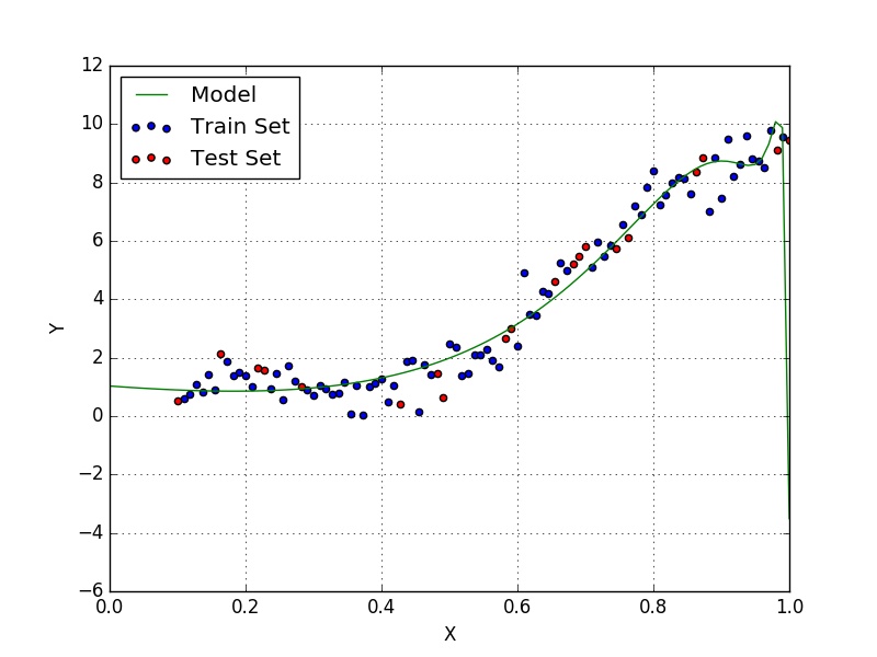
In this tutorial we will be fitting a higher order polynomial to the same dataset used in the previous text using stochastic gradient descent. In the end our model will be producing results similar to Fig. 1.
Stochastic Gradient Descent
Stochastic Gradient Descent (SGD for short) is a flavor of Gradient Descent which uses smaller portions of data (mini batches) to calculate the gradient at every step (in contrast to Batch Gradient Descent, which uses the entire training set at every iteration). This allows us to efficiently work with bigger data sets, which otherwise we would not be able to fit in RAM entirely and therefore would make vectorization much less efficient. The algorithm now becomes:
until stopping criteria:

    shuffle training set

    for mini-batch $\boldsymbol{\in}$ training set

    1. Evaluate gradients using mini-batch

    2. Update parameters by $P = P - \alpha \dfrac{\partial\mathcal{L}(y,x,P)}{\partial P}$
Notice that although we use mini-batches at each iteration, we still go through the entire data set and every time we do so we complete an epoch. The stochasticity also helps in converging to the global minimum in non-convex optimization, since the noise in calculating the gradient from different mini batches might pull the parameters from a local minimum. For convex optimization problems, however, batch gradient descent has faster convergence since it always follows the patch of steepest descent.
Code
To code multiple linear regression we will just make adjustments from our previous code, generalizing it. For this tutorial we will be fitting the data to a fifth order polynomial, therefore our model will have the form shown in Eq. $\eqref{eq:poly}$.
Setup
We initialize our data the same way we did before, except now we pre-compute each feature vector (the powers of the input, in this case) and normalize along each feature.
import numpy as np

model_order = 6 # Polynomial order + Intersect

data_x = np.linspace(1.0, 10.0, 100)[:, np.newaxis]
data_y = np.sin(data_x) + 0.1*np.power(data_x,2) + 0.5*np.random.randn(100,1)

data_x = np.power(data_x, range(model_order))
data_x /= np.max(data_x, axis=0)
We then proceed to segment our training and test sets the same way we did before.
order = np.random.permutation(len(data_x))
portion = 20
test_x = data_x[order[:portion]]
test_y = data_y[order[:portion]]
train_x = data_x[order[portion:]]
train_y = data_y[order[portion:]]
Error and Gradient
Our error and gradient functions will remain the same since our loss function is still the squared error and the different powers of the input are pre-computed, therefore appear as simply more features to our model. We repeat the code here for completeness.
def get_gradient(w, x, y):
    y_estimate = x.dot(w).flatten()
    error = (y.flatten() - y_estimate)
    mse = (1.0/len(x))*np.sum(np.power(error, 2))
    gradient = -(1.0/len(x)) * error.dot(x)
    return gradient, mse
Stochastic Gradient Descent
We can now implement our stochastic gradient descent routine.
w = np.random.randn(model_order)
alpha = 0.5
tolerance = 1e-5

# Perform Stochastic Gradient Descent
epochs = 1
decay = 0.95
batch_size = 10
iterations = 0
while True:
    order = np.random.permutation(len(train_x))
    train_x = train_x[order]
    train_y = train_y[order]
    b=0
    while b < len(train_x):
        tx = train_x[b : b+batch_size]
        ty = train_y[b : b+batch_size]
        gradient = get_gradient(w, tx, ty)[0]
        error = get_gradient(w, train_x, train_y)[1]
        w -= alpha * gradient
        iterations += 1
        b += batch_size

    # Keep track of our performance
    if epochs%100==0:
        new_error = get_gradient(w, train_x, train_y)[1]
        print "Epoch: %d - Error: %.4f" %(epochs, new_error)

        # Stopping Condition
        if abs(new_error - error) < tolerance:
            print "Converged."
            break

    epochs += 1
    alpha = alpha * (decay ** int(epochs/1000))
First we initialize our weight vector and our hyperparameters (learning rate, decay rate, tolerance and mini-batch size). Then we start our actual stochastic gradient descent loop, first we shuffle our training set then we go through it in mini-batches of 10 samples. Notice that now we also use a different stopping condition: This time we halt training when our error changes less than a certain threshold between epochs, for no reason other than illustrative purposes. Finally, we also implement learning rate decay (last line of code), which consists of decreasing the learning rate as the training proceeds. We do so using Eq. $\eqref{eq:alpha_decay}$, notice that we use a very mild decay rate.
Results
With this model we get a training error of 0.3126 (75% smaller than simple linear regression) and test error of 0.3403 (85% smaller). Our final model is shown in Eq. $\eqref{eq:poly_trained}$.
Overfit
From the decrease in test error perceived from the simple model to the new one you might think that it is a good idea to keep increasing the order of the model. This is not a good idea, however, as it might lead to overfitting, which is a phenom that happens when the model starts to fit the peculiarities of the training set (i.e. make an effort to fit outliers in the set). In Fig. 2 we can see that the model shows a form which is unlikely to be the true behaviour of the data we are modelling.
This subject will be of particular interest to us when we discuss neural networks, especially convolutional neural networks. We will also see ways of avoiding and remeding it.
Jupyter notebook available here
Last modified: May 29, 2016 comments powered by Disqus