Introduction

The problem of classification consists in assigning an observation to the category it belongs. That means, for instance, taking a picture of a handwritten digit and correctly classifying which digit (0-9) it is, matching pictures of faces to whom they belong or classifying the sentiment in a text. In general, when dealing with classification we use supervised learning (when we have an annotated training set from which we can learn our model - as we did up until this point). In unsupervised learning we can do clustering, where we have no notion of classes, but instead we have clusters of data points that share similar features, we shall be seeing these models in future articles.

Geometrically, the task consists of finding a hyperplane (or set of hyperplanes, which are spaces one dimension smaller than the ambient space, i.e. a line is a hyperplane in a 2D space) that separates the data points of each class. Fig. 1 illustrates the process of finding a hyperplane, notice that in the end you have a line (decision boundary) that separates the blue points from the red.

One method of tackling classification problems is Logistic Regression, which is a specialized case of the linear regression, differing in the sense that logistic regression maps its input into a class by applying a sigmoid function. So if our model of linear regression is $y = w^Tx+b$, then logistic regression is $y = \sigma(w^Tx+b)$ where $\sigma(x) = \dfrac{1}{1+e^{-x}}$. Notice that the sigmoid function produces values in the range (0,1), which makes the interpretation as a probability convenient. If you’re somewhat familiar with Neural Networks, notice that logistic regression is nothing more than a single layer ANN.

One-Hot Encoding

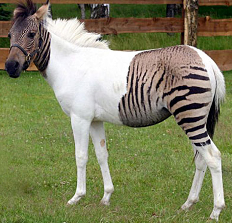
Before we can actually dive into logistic regression, we must first reflect about how to encode a class. So far our functions have produced values in $\mathbb{R}$, so an immediate idea is to assign a class to each number. For instance, we could encode “Zebra” as 0 and “Horse” as 1 (“Lion” as 2, “Gazelle” as 3 and so on…). However, this raises the question of what the median values mean, is 0.5 a Zorse?

To solve this problem we use one-hot encoding, which consists of using a N-dimensional vector to encode N classes, where at any time only one dimension has high value (1), while all the others have low (0). So in our previous example we would have $\text{Zebra} = [1,0,0,0]$, $\text{Horse} = [0,1,0,0]$, and so on.

Softmax Function

If we want to use one-hot encoding we need to generalize the sigmoid function to multiple classes, otherwise we would be constrained to only performing binary classification. For this purpose we have the Softmax Function, which is a generalization of the sigmoid function for higher dimensions, while still keeping the neat property of summing up to one and therefore being interpretable as a probability. Given a K-dimensional class space, we have the Softmax function shown in Eq. 1.

Negative Log-Likelihood Cost

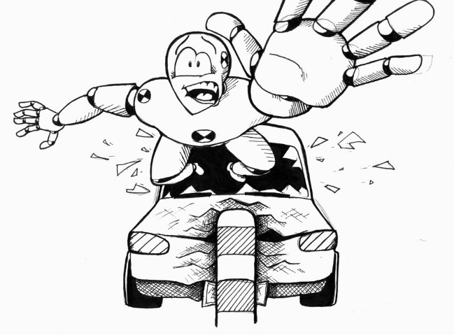
Given this new encoding we need a new objective function since squared-error would just pull us towards an average of all classes. So for instance if you’re teaching an autonomous vehicle to choose between turning left and right and use squared error loss, when in doubt between left and right it will just go straight ahead (and crash).

Using the Negative Log-Likelihood (NLL) cost, however, we drive the model towards choosing a single class for each input. In other words, we want to maximize the likelihood of our model parameters ($\theta$) correctly predicting the class ($y$) of every data point ($x$) in a D-dimensional class space (D classes).

Notice in Eq. 2 that for the purposes of maximization we don’t care about $P(x | \theta)$, therefore we can reduce it to:

It is more convenient for us to work in log domain, therefore we arrive at the cost function shown in Eq. .

MNIST

For the coding part of this article we will be classifying pictures of handwritten digits from MNIST (with some samples shown in Fig. 4), which is one of the most widely used datasets in machine learning.

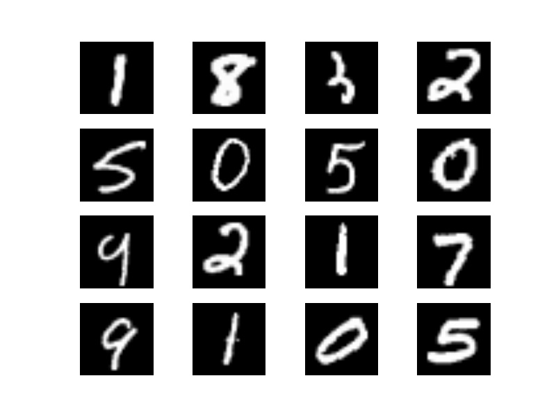
Our dataset will consist of 55,000 training, 10,000 test and 5,000 validation points. For purposes of comparison, state of the art models achieve error rates as low as 0.25% in this data.

Code

As usual, we start by loading the appropriate packages.

import numpy as np
import matplotlib.pyplot as plt
import tensorflow as tf

We then proceed to load the MNIST dataset, which comes bundled with TensorFlow. Feel free to change ”/tmp/data/” to another directory if you wish.

from tensorflow.examples.tutorials.mnist import input_data
mnist = input_data.read_data_sets("/tmp/data/", one_hot=True)

Model

We now code our model graph much in the same way we did for linear regression.

init_param = lambda shape: tf.random_normal(shape, dtype=tf.float32)

with tf.name_scope("IO"):
    inputs = tf.placeholder(tf.float32, [None, 784], name="X")
    targets = tf.placeholder(tf.float32, [None, 10], name="Yhat")

with tf.name_scope("LogReg"):
    W = tf.Variable(init_param([784, 10]), name="W")
    B = tf.Variable(init_param([10]))
    logits = tf.matmul(inputs, W) + B
    y = tf.nn.softmax(logits)

Notice here the dimension of the parameters. MNIST has images of size 28x28, which have to be flattened before being fed to the model, becoming a 784x1 vector. Also, we are dealing with 10 classes, therefore our parameters have to reflect these dimensions, w has to take a $\mathbb{R}^{784}$ vector and output a $\mathbb{R}^{10}$ vector, therefore it has to be a 784x10 matrix. b has to sum with this vector, therefore it must have the same length (10x1). Finally, we compute the softmax of our logits ($wx+b$).

Now we can define our objective function and other metrics. TensorFlow already has a negative log-likelihood cost (same as cross entropy) implemented, so we use it. We also implement an accuracy calculation which simply compares our highest ranking class against the ground truth in order to evaluate our model.

with tf.name_scope("train"):
    learning_rate = tf.Variable(0.5, trainable=False)
    cost_op = tf.nn.softmax_cross_entropy_with_logits(logits, targets)
    cost_op = tf.reduce_mean(cost_op) 
    train_op = tf.train.GradientDescentOptimizer(learning_rate).minimize(cost_op)
    
    correct_prediction = tf.equal(tf.argmax(y, 1), tf.argmax(targets,1))
    accuracy = tf.reduce_mean(tf.cast(correct_prediction, tf.float32))*100

Train

From there, our training routine is pretty standard, much likely we have been implementing so far. With the exception that here we use the built-in functions from the MNIST dataset to create and load the mini-batches.

tolerance = 1e-4

# Perform Stochastic Gradient Descent
epochs = 1
last_cost = 0
alpha = 0.7
max_epochs = 100
batch_size = 50
costs = []
sess = tf.Session()
print "Beginning Training"
with sess.as_default():
    init = tf.initialize_all_variables()
    sess.run(init)
    sess.run(tf.assign(learning_rate, alpha))
    writer = tf.train.SummaryWriter("/tmp/tboard", sess.graph) # Create TensorBoard files
    while True:

        num_batches = int(mnist.train.num_examples/batch_size)
        cost=0
        for _ in range(num_batches):
            batch_xs, batch_ys = mnist.train.next_batch(batch_size)
            tcost, _ = sess.run([cost_op, train_op], feed_dict={inputs: batch_xs, targets: batch_ys})
            cost += tcost
        cost /= num_batches

        tcost = sess.run(cost_op, feed_dict={inputs: mnist.test.images, targets: mnist.test.labels})
            
        costs.append([cost, tcost])
        
        # Keep track of our performance
        if epochs%5==0:
            acc = sess.run(accuracy, feed_dict={inputs: mnist.train.images, targets: mnist.train.labels})
            print "Epoch: %d - Error: %.4f - Accuracy - %.2f%%" %(epochs, cost, acc)

            # Stopping Condition
            if abs(last_cost - cost) < tolerance or epochs > max_epochs:
                print "Converged."
                break

            last_cost = cost
            
        epochs += 1
    
    tcost, taccuracy = sess.run([cost_op, accuracy], feed_dict={inputs: mnist.test.images, targets: mnist.test.labels})
    print "Test Cost: %.4f - Accuracy: %.2f%% " %(tcost, taccuracy)

Results

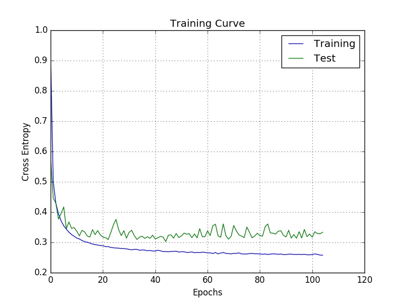
After 105 epochs we are at a train accuracy of 92.99% and test accuracy of 91.60%. These results may appear impressive but they’re actually shamefully low, when we tackle this dataset again using a convolutional neural network we should be able to get accuracies in the upper 99 percentages. If we plot curve of cost against the number of epochs we arrive at Fig. 5, notice how both the train and test costs reduce at first and then the training costs starts decreasing very slowly while the test just oscillates around the same mean. At this point we may just halt training since the model is no longer learning useful features, but instead is just fitting peculiarities of the training set. In fact, one of the methods of avoiding overfitting is based exactly in this thinking - Early Stopping - which attempts to detected when the test cost stops decreasing and halts training, both saving us time and providing us with a better model.

As usual, in Fig. 6 we can see how the model behaves as we train it. As we expected, after just a few epochs it already gets most classes right.