Introduction

Linear regression is a method used to find a relationship between a dependent variable and a set of independent variables. In its simplest form it consist of fitting a function $ \boldsymbol{y} = w.\boldsymbol{x}+b $ to observed data, where $\boldsymbol{y}$ is the dependent variable, $\boldsymbol{x}$ the independent, $w$ the weight matrix and $b$ the bias.

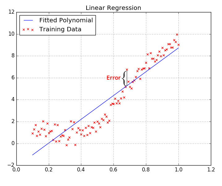
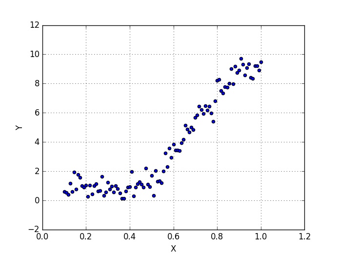
Illustratively, performing linear regression is the same as fitting a scatter plot to a line. As can be seen for instance in Fig. 1.

Background

Before we can broach the subject we must first discuss some terms that will be commonplace in the tutorials about machine learning. They are:

Hyperparameters

In statistics hyperparameters are parameters of a prior distribution. In our case it relates to the parameters of our model (the number of layers in a neural network, the number of neurons in each layer, the learning rate, regularization, etc.). The concept will become clear as we discuss some models.

Loss Function

A loss function is a way to map the performance of our model into a real number. It measures how well the model is performing its task, be it a linear regression model fitting the data to a line, a neural network correctly classifying an image of a character, etc. The loss function is particularly important in learning since it is what guides the update of the parameters so that the model can perform better.

Train, Validation, Test

It is usually a good idea to partition the data in 3 different sets: Train, Validation and Test. Each of them serving a different purpose:

• Train set is used to actually learn the model. The data is presented to the model and the learning method produces a fit.
• Validation set is used to tune the hyperparameters.
• Test set is used to evaluate the overall performance of the model.

Its important that these sets are sampled independently so that one process does not interfere with the other. If we estimated the performance of the model according to the train set we would get a artificially high value because those are the data points used to learn the model.

Error Function

In order to estimate the quality of our model we need a function of error. One such function is the Squared Loss, which measures the average of the squared difference between an estimation and the ground-truth value. Given Fig. 1, for instance, the squared loss (which we will refer to henceforth as MSE - Mean Squared Error) would be the sum of square of the errors (as shown) for each training point (the xs), divided by the amount of points. A good intuition for the squared loss is that it will drive the model towards the mean of the training set, therefore it is sensitive to outliers. The squared loss function can be seen in Eq. $\eqref{eq:sq_loss}$, where $M$ is the number of training points, $y$ is the estimated value and $\hat{y}$ is the ground-truth value.

We can further expand Eq. $\eqref{eq:sq_loss}$ in order to incorporate our model. Doing so we obtain Eq. $\eqref{eq:model_loss}$.

Naturally, we want a model with the smallest possible MSE, therefore we’re left with the task of minimizing Eq. $\eqref{eq:model_loss}$.

Gradient Descent

One of the methods we can use to minimize Eq. $\eqref{eq:model_loss}$ is Gradient Descent, which is based on using gradients to update the model parameters ($w$ and $b$ in our case) until a minimum is found and the gradient becomes zero. Convergence to the global minimum is guaranteed (with some reservations) for convex functions since that’s the only point where the gradient is zero. An animation of the Gradient Descent method is shown in Fig 2.

Taking the gradients of Eq. $\eqref{eq:model_loss}$ (the derivatives with respect to $w$ and $b$) yields Eqs. $\eqref{eq:dl_dw}$ and $\eqref{eq:dl_db}$.

Remember from calculus that the gradient points in the direction of steepest ascent, but since we want our cost to decrease we invert its symbol, therefore getting the Eqs. 5 and 6:

Where $\alpha$ is called learning rate and relates to much we trust the gradient at a given point, it is usually the case that $0 < \alpha < 1$. Setting the learning rate too high might lead to divergence since it risks overshooting the minimum, as illustrated by Fig. 3.

The Algorithm

The batch gradient descent algorithm works by iteratively updating the parameters using Eqs. 5 and 6 until a certain stopping criteria is met.

until stopping criteria:

1. Evaluate gradients
2. Update parameters by $P = P - \alpha \dfrac{\partial\mathcal{L}(y,x,P)}{\partial P}$

There are many flavours of Gradient Descent, with the explained above being the simplest (and slowest) among them, in the following posts we will be discussing variants of it, with some of them being illustrated in Fig. 4.

The Code

Having briefly talked about the theory we can now start coding our model. In this and following guides we will be using Python 2.7 and NumPy, if you don’t have them installed I recommend using Conda as a package and environment manager, Jupyter/IPython might come in handy as well.

Data

First we load the necessary packages and generate some data:

import numpy as np

data_x = np.linspace(1.0, 10.0, 100)[:, np.newaxis]
data_y = np.sin(data_x) + 0.1*np.power(data_x,2) + 0.5*np.random.randn(100,1)
data_x /= np.max(data_x)

Notice that we divide data_x by its maximum value, that is called normalization and it helps in keeping the algorithm numerically stable. Our data right now can be seen in Fig. 5.

In order to simplify our model we use a trick which consists in including the intercept in the input values, this way we dont have to carry the bias ($b$) term through the calculation, that’s done by adding a column of ones to the data, this way our model becomes simply $y = w^Tx$.

data_x = np.hstack((np.ones_like(data_x), data_x))

We now shuffle and segment our data in training and test sets. No need for a validation set here since we have no intention of tuning hyperparameters.

order = np.random.permutation(len(data_x))
portion = 20
test_x = data_x[order[:portion]]
test_y = data_y[order[:portion]]
train_x = data_x[order[portion:]]
train_y = data_y[order[portion:]]

Error and Gradient

Lets now code our error (Eq. $\eqref{eq:model_loss}$) and gradient (Eqs. $\eqref{eq:dl_dw}$ and $\eqref{eq:dl_db}$) functions. Notice that since we’ll be multiplying it by the learning rate we don’t actually need to multiply by two. Notice too how the implementation makes no use of for-loops, performing the calculations using matrix multiplications instead, this promotes great speedups. In fact, when using math libraries such as NumPy you should always try to produce good, vectorized code since their functions are optimized to perform matrix multiplications (but don’t take my word for it - look up BLAS).

def gradient(w, x, y):
    y_estimate = x.dot(w).flatten()
    error = (y.flatten() - y_estimate)
    gradient = -(1.0/len(x)) * error.dot(x)
    return gradient, np.pow(error, 2)

Gradient Descent

We can now code our actual gradient descent loop.

w = np.random.randn(2)
alpha = 0.5
tolerance = 1e-5

# Perform Gradient Descent
iterations = 1
while True:
    gradient, error = get_gradient(w, train_x, train_y)
    new_w = w - alpha * gradient
    
    # Stopping Condition
    if np.sum(abs(new_w - w)) < tolerance:
        print "Converged."
        break
    
    # Print error every 50 iterations
    if iterations % 100 == 0:
        print "Iteration: %d - Error: %.4f" %(iterations, error)
    
    iterations += 1
    w = new_w

We first initialize our weight matrix ($w$) with two random values (initializing with zeros is fine as well), set our learning rate ($\alpha$) and define our tolerance, which will define our stopping criteria later. Inside the loop we calculate the gradient and error for the current model and update the weight matrix, we then check if the sum of the absolute differences between the new and old values is bigger than our tolerance (or, in other words, if our model changed significantly).

Results

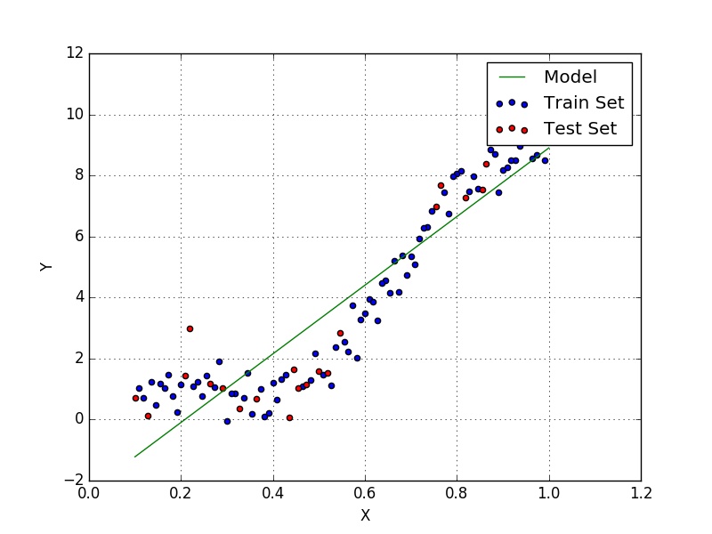
At the end we get a training error of 1.2636 and $w = [-2.3436, 11.2450]$ (shown in Fig. 7). If we compute the error against the test set we get a value of 2.1382, notice that it is slightly larger than the training set, since we’re comparing the model to data that it hasn’t been exposed to.

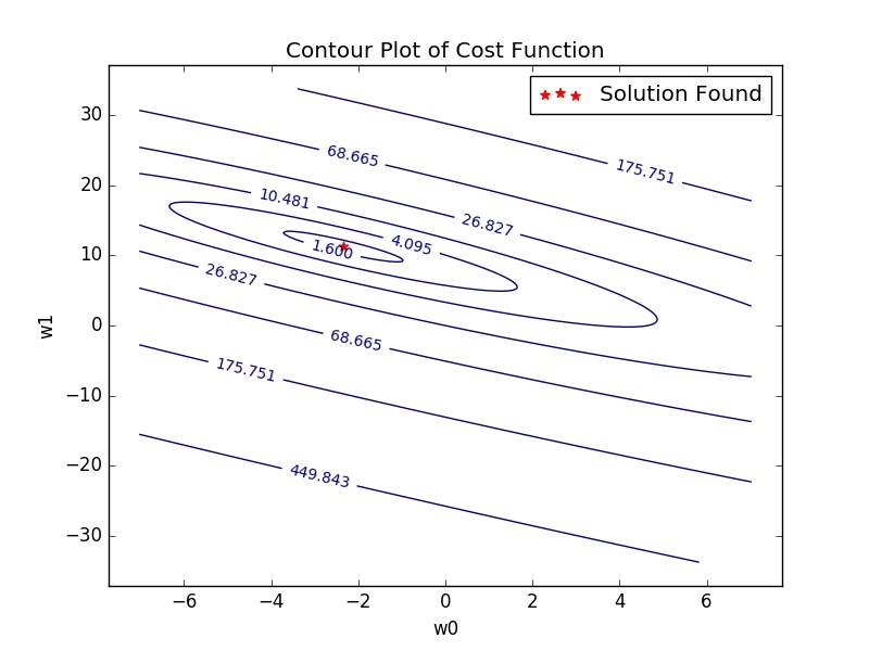
Making a contour plot of the error function and our results yields Fig. 8, which shows that we have reached a minimum (in fact the global minimum, since it can be shown that our loss function is convex).

In the next tutorial we’ll talk about multiple linear regression, which consists of a simple extension to our model that allows us to use multiple descriptive variables to predict the dependent variable, effectively allowing us to model higher order polynomials (i.e. $y = \sum_{i=0}^{k} w_ix^i$).