

Introduction to Image Segmentation
Jump to Image Segmentation: Introduction | SE Min-Cut | Results | Benchmarking | Publication | References, or Research Overview.
Humans can often identify salient structures in an image, even when they have no idea what they are looking at. As Witkin and Tenenbaum wrote[1]:
What is remarkable is the degree to which such naively perceived structure survives more or less intact once a semantic context is established... It is almost as if the visual system has some basis for guessing what is important without knowing why.
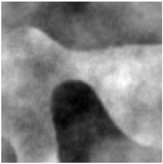
Here we consider the case of perceiving salient subregions of an image. For example, given the top-left image below, we might naturally divide it into the differently coloured large regions shown on the bottom-right panel. These regions represent our guess for what is important in the image, but we don't really know why.
| ||||||||||

In the field of computer vision the "image segmentation problem" typically refers to the partitioning of the whole image into a small set of distinct and (probably) salient components (e.g. bottom-right image above). The more far-reaching goal here is that would like to be able to use the resulting regions as part of the input for a subsequent object identification stage. Therefore, at this earlier stage, we want to avoid making assumptions on what objects are present. That is, we want to try guessing which regions are important without yet knowing why, and then use these guessed regions to help decide which objects are present.
Note that, in the Fractals image, the edges between the large regions are often clearly visible in the original image, but there are also places where these edge either vanish or become much less distinct. We refer to these relatively indistinct boundary segments as "leaks". For example, there is a leak between the royal blue and green regions near the top-left corner of the Fractals image. Similarly, the boundary between the green and grey-blue regions has a leak near the bottom-right corner.
A key property of a suitable segmentation algorithm is that it is capable of ignoring such leaks between salient regions. The use of a minimum-cut approach, as described next, appears to be a useful tool for dealing with leaks.
A general class of image segmentation algorithms use a graph representation for an image. In this graph each pixel is represented by a vertex. The (undirected) edges in this graph link neighbouring pixels and have weights that represent the pixel similarities (see below, and ignore for now the distinction between red and black edge weights). That is, neighbouring pixels which have more similar RGB values have higher weights on their associated edges.
|
A segmentation is simply an assignment of pixels to segment labels. One possible measure of the "cost" of a segmentation is the standard cut cost defined in graph theory. That is, the "cut cost" of a segmentation is taken to be the sum of the weights of all those edges which connect two pixels having different labels.
For example, in the 4x4 image above, the segmentation of the center 2x2 square from the background causes exactly those edges which have their cost shown in red to be cut. The sum of these red edge weights gives a cut cost of 33. This appears to be the minimum-cost segmentation for this image. This is intriguing because the center 2x2 region also seems like a good guess for what is important in this image.
Unfortunately, a minimum cut segmentation does not always give plausible regions. For example, if we changed the top-left horizontal edge to have a similarity of 12 instead of 15 then the minimum cut would then be to separate the top left pixel from the rest of the graph. The resulting segmentation has a cut cost of 20+12=32, instead of 33, but does not seem visually important.
In fact, it is relatively common for the minimum cut of the pixel graph of typical images to simply separate a small collection of pixels from the rest of an image. This issue is discussed by Shi and Malik[2] and it led to their proposal for the Normalized Cut (NCut) algorithm.

Jump to Image Segmentation: Introduction | SE Min-Cut | Results | Benchmarking | Publication | References, or Research Overview.
The SE Min-Cut Algorithm. We have developed an approach to image segmentation called Spectral Embedding Min-Cut (SE Min-Cut). An illustration of some intermediate steps within the SE Min-Cut algorithm is given in the Fractals figure above.
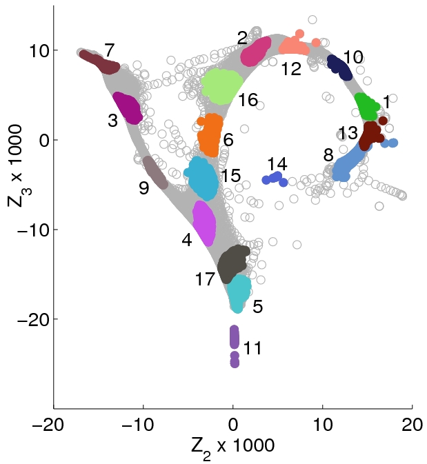
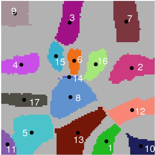
The first step of SE Min-Cut is to use a spectral embedding of the pixel graph (weighted by similarities) to do a soft clustering of the pixels. The top-right image in the Fractals figure shows a two dimensional projection of the spectral embedding, where each pixel is represented as a circular data point. This embedding has the property that pixels which are considered to be similar (according to the weighted graph) are mapped close to one another, while dissimilar pixels are placed further apart. So called "seed regions" are then computed by computing tight clusters of pixels within the spectral embedding. We indicate the correspondence between seed regions in the embedding with the same pixels in the original image frame by using the same colouring and numbering for both sets (see bottom-left panel in Fractals figure).
In these plots notice how the connection between locally similar regions in the original image appear to be associated with densely populated regions in the embedding (e.g., regions 2 and 12). Conversely, dissimilar neighbouring regions in the image can be seen to be separated by a much more sparsely populated region in the embedding (e.g., regions 2 and 7).
Given the seed regions, the algorithm proceeds by using a graph algorithm for ST min-cut problems to find boundaries between various subsets of seed regions. The union of all these boundaries is considered, and this typically results in an oversegmentation of the image. Finally, region merging is used to form the final segmentation. The result for the Fractals image is shown in the bottom-right panel. See the BMVC 2004 paper below for details of this algorithm.
Jump to Image Segmentation: Introduction | SE Min-Cut | Results | Benchmarking | Publication | References, or Research Overview.
Results. The figure below shows the segmentation results of the SE-MinCut and several other algorithms on synthetic fractal images.
 |
Details of the other segmentation algorithms cited above are available from the references: NCut [2] and [3]; Local Variation [4]; and Mean Shift [5].
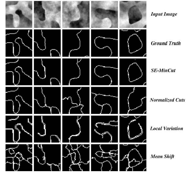
Example segmentations for images from the Berkeley segmentation database [6] are shown below.
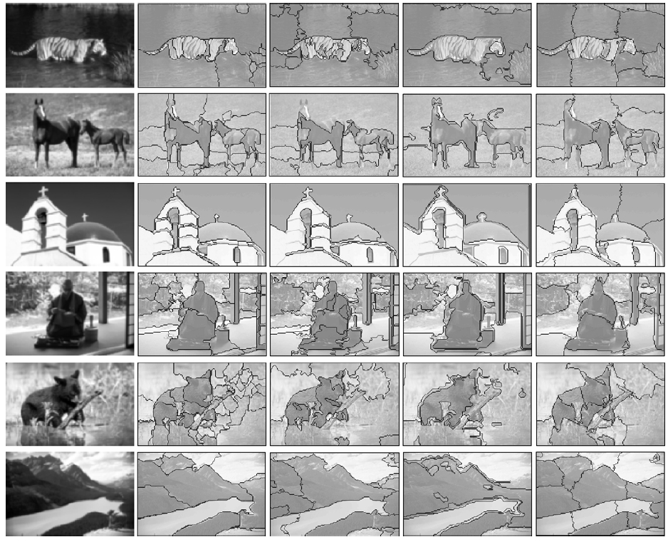 |
The segmentation algorithms used in the second through fifth column above are, respectively, SE Min-Cut, Mean Shift [5], Local Variation [4], and NCut [3].
Jump to Image Segmentation: Introduction | SE Min-Cut | Results | Benchmarking | Publication | References, or Research Overview.
A quantitative comparison of these same segmentation algorithms is provided in our benchmarking paper. The prediction recall curves obtained for a set of synthetic fractal images are shown below.
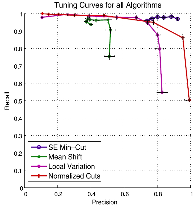 |
This plot indicates that the segmentations produced by the SE Min-Cut algorithm agree fairly well with the ground truth segmentations for this particular set of synthetic fractal images. The performance of the NCut algorithm is also quite good.
The predicition-recall curves obtained for the Berkeley image database are shown below.
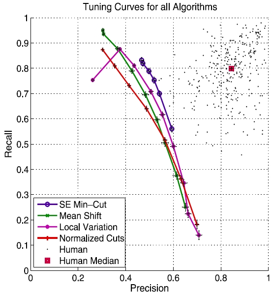 |
The SE min-cut algorithm again provides somewhat better precision-recall results. However, here the local variation (LV) algorithm comes next. This performance of LV is interesting in that it is significantly faster than the other algorithms.
The black dots in the above plot provide comparisons of the segmentations provided by different humans, which are available from the Berkeley database and are used for the ground truth in the above prediction-recall plot. We conclude that the humans agree on their image segmentations with other humans to a greater degree than humans agree with any of these segmentation algorithms.
Note that, for each individual algorithm, there is a significant change in the precision-recall curve across the two datasets, that is, between synthetic fractal images on the one hand and natural images from the Berkeley database on the other. All the algorithms find the Berkeley dataset significantly harder.
This change could be due to the fact that the ground truth in the Berkeley database is based on image segmentations done by humans. It is plausible that these human subjects used object specific information to arrive at their segmentations, which the algorithms do not have access to.
Another possible factor in the change in the precision-recall curves across the two datasets is a difference in the image structure itself. Natural images are generated from scenes consisting of different 3D objects, with different classes of textures and pigmentation, along with significant variations in lighting. However, the fractal image set has a much more limited range of effects.
An interesting project would be to create alternative synthetic segmentation databases with more natural image structure and objective segmentations. If the precision-recall curves stay high, even for much more natural looking images, then this would support the hypothesis that object or scene specific information may be significant in the human segmentations of the Berkeley dataset.
Jump to Image Segmentation: Introduction | SE Min-Cut | Results | Benchmarking | Publication | References, or Research Overview.
F. J. Estrada, and A. D. Jepson, Benchmarking Image Segmentation Algorithms, International Journal of Computer Vision, Vol. 85, No. 2, p. 167, 2009. PDF (1306KB) Also see Segmentation Evaluation and Benchmarking.
F. J. Estrada, A. D. Jepson, and C. Chennubhotla, Spectral Embedding and Min-Cut for Image Segmentation, British Machine Vision Conference, London, U. K., 2004. PDF (1371KB)
Jump to Image Segmentation: Introduction | SE Min-Cut | Results | Benchmarking | Publication | References, or Research Overview.
References.
[1] A.P. Witkin and J.M. Tenenbaum, On the role of structure in vision, in Human and Machine Vision, ed. A. Rosenfeld, Academic Press, 1983, p.481.
[2] Jianbo Shi and Jitendra Malik, Normalized Cuts and Image Segmentation, IEEE Transactions on Pattern Analysis and Machine Intelligence(PAMI), 2000.
[3] T. Cour, S. Yu, and J. Shi, (2006). Normalized cuts Matlab code, Computer and Information Science, Penn State University.
[4] P. Felzenszwalb, and D. Huttenlocher, (2004). Efficient Graph-Based Image Segmentation, International Journal of Computer Vision, Volume 59, Number 2.
[5] C.M. Christoudias, B. Georgescu, and Peter Meer, Synergism in low level vision, 16th Int. Conf. on Computer Vision, 2002. Code for EDISON system.
[6] D. Martin and C. Fowlkes and D. Tal and J. Malik, A Database of Human Segmented Natural Images and its Application to Evaluating Segmentation Algorithms and Measuring Ecological Statistics, Proc. 8th Int. Conf. Computer Vision, 2001, pp.416-423. See also the Berkeley segmentation database and benchmark
Jump to Image Segmentation: Introduction | SE Min-Cut | Results | Benchmarking | Publication | References, or Research Overview.
