CSC411: Study Guide

CSC411 Study Guide, Winter 2017 (Last update: 04/02/17.)

Suppose our training set and test set are the same. Why would this be a problem?
Why is it necessary to have both a test set and a validation set?
Images are generally represented as $n\times m\times 3$ arrays, but we treat them as vectors. How is that possible?
Write pseudocode to select the $k$ in the $k$ -nearest-neighbours algorithm.
Give an example of a training and a test set such that 3-nearest-neighbours and 5-nearest neighbours perform differently on the test set.
Consider the data plotted below. If all that you have to go by is the data below, how would you objectively determine whether 1-NN or 15-NN is the better classifier for the data?
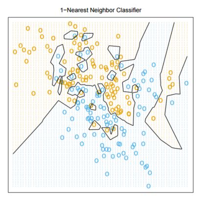
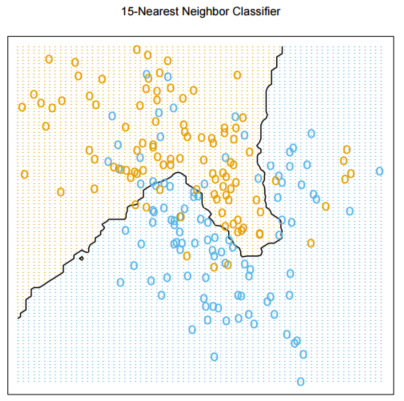
What is the performance of k-NN on the training set for k = 1? Is it the same for k = 3? (Give an example in your answer to the second question.)
What happens to the performance of k-NN if k is the same as the size of the training set?
Explain why the negative cosine distance may make more sense for comparing images than the Euclidean distance.
Give an example of a dataset where the Euclidean distance metric makes more sense than the negative cosine distance.
Explain how the quadratic cost function
$$J(\theta_0, \theta_1) = \frac{1}{2m} \sum_{i}^{m}(h_\theta(x^{(i)})-y^{(i)})^2 $$
is constructed. Specifically, what is the intuitive meaning of $(h_\theta(x^{(i)})-y^{(i)})^2$ ?
How to estimate the best $h_{\theta}$ by looking at a surface plot of the cost function?
How to estimate the best $h_{\theta}$ by looking at a contour plot of the cost function?
Write a Python function to find a local minimum of $y = x^6 - 10 x^5- 5x^4 + 1$ using gradient descent.
On a plot of a function of one variable $y= f(x)$ , at point $(x_0, f(x_0))$ , write down a unit vector that points “uphill.”
On a surface plot of a function of two variables, at point $(x_0, y_0, f(x_0, y_0))$ , write down a unit vector that points “downhill.”
With Gradient Descent, desribe functions for which a larger $\alpha$ makes sense, and functions for which a lower $\alpha$ makes sense. Use sketches of the functions.
Without computing the gradient symbolically, how can you estimate it? (Hint: generalize the technique we used for computing $\partial f/\partial x_i$ to check that the gradient computation was correct.
Suppose $J(\theta)$ is the cost function for linear regression. Explain how to interpret $\partial J/\partial \theta_0 = 1/m \sum_i (\theta^T x^{(i)}-y^{(i)})$ , where $\theta_0$ is the constant coefficient.
Explain how to use regression in order to solve two-classification problems. What’s the problem with using this approach for multi-class classification?
Describe a technique for using regression for multi-class classification problems.

Show that the code below computes the gradient with respect to the parameters of a linear hypothesis function

def df(x, y, theta):
    x = vstack( (ones((1, x.shape[1])), x))
    return -2*sum((y-dot(theta.T, x))*x, 1)

Write non-vectorized code to perform linear regression.
Explain how points that are not separable by a linear decision boundary using just the original features can become separable by a linear decision boundary if computed features are used.
When converting a classification problem into a regression problem, we assigned the output 1 Class A and the output 0 to Class B. We then predicted y = 1 for $h_{\theta}(x) > .5$ . If it’s more expensive to mistakenly predict that y = 1 when it’s actually 0 than vice versa, we can decide to predict y = 1 for $h_{\theta}(x) > .7$ . Explain why that is, using a concrete numerical example.
Recall that we can find the Maximum Likelihood solution to linear regression problems using $\hat{\theta} = (X^T X)^{-1} (X^T Y)$ . Suppose you are given a dictionary paul_imgs whose keys are 0..19 , and a dictionary john_imgs whose keys are 0..19 such that paul_imgs[i] and john_imgs[i] are the i-th image of Paul and John, respectively. The images are $20\times 20$ NumPy arrays representing grayscale images. Write NumPy code that would take in a new image, and return True if it’s likely a picture of Paul and False if it’s likely a picture of John. Use linear regression.
Explain why it makes sense to use Maximum Likelihood estimation.
Explain why it sometimes makes sense to use a prior on the parameter $\theta$ .
Show that, for priors that are never zero, the more training data there is, the less important is the prior for Maximum A-Posteriori inference. Show that by writing down the posterior probability that is being maximized

Recall the following code. Explain why theta_hat will tend to have larger values (in terms of the absolute value than theta .

def compare_theta_theta_hat(N, ndim, sigma_theta, sigma):
    theta = scipy.stats.norm.rvs(scale=sigma_theta,size=ndim+1)

    x_raw = 100*(random.random((N, ndim))-.5)

    x = hstack((ones((N, 1)),
        x_raw,
        ))

    y = dot(x, theta) + scipy.stats.norm.rvs(scale= sigma,size=N)

    theta_hat = dot(linalg.pinv(dot(x.T, x)), dot(x.T, y))

    return theta[1], theta_hat[1]

How would you use Bayesian inference in order to make it so that theta_hat is not systematically larger? Explan why your prior makes sense.
Show that minimizing the sum of squared differences between the prediction $h_\theta (x)$ and the actual outputs $y$ is equivalent to maximizing the likelihood when $y\sim N(\theta^T x, \sigma^2)$ .
Show how to compute AND using a neural network that uses logistic neurons.
Why can’t you use the log-loss when using linear neurons?
Assume that $y\sim Poisson(\theta^T x)$ . Derive the log-likelihood of the training set where the inputs are x and the output are y.
Write Python code to find the Maximum Likelihood estimate for $\theta$ where $y\sim Poisson(\theta^T x)$ .
After you find the Maximum Likelihood estimate for $\theta$ where $y\sim Poisson(\theta^T x)$ , how would you use it to make predictions for new data?
Suppose that your model for the data is
$$y\sim Poisson(\alpha x+10), $$
with $\alpha \in \mathbb{R}$ . Assume you believe that $\alpha\sim N(0, \beta)$ . Write Python code to obtain the posterior distribution of $\alpha$ given a dataset, and to obtain the Maximum A-Posteriori (MAP) estimate of $\alpha$ .
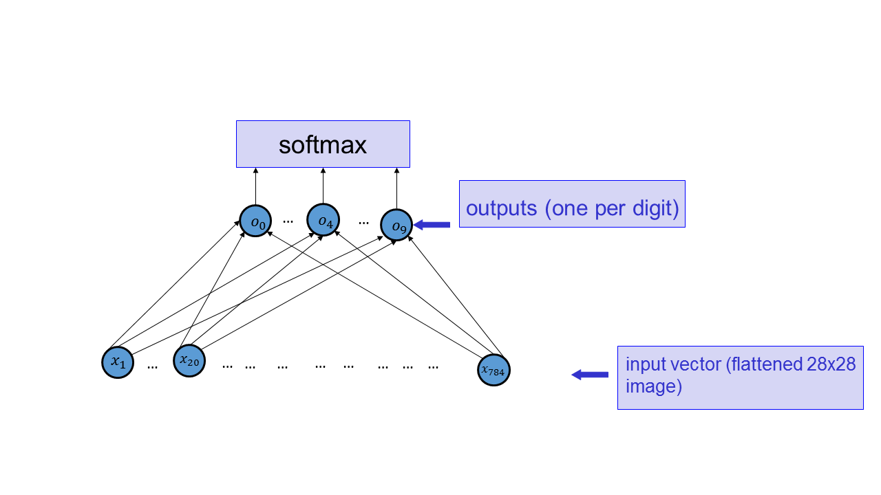
Write vectorized code (i.e., you cannot use for-loops) to compute the output of a feedforward neural network with the activation function $g$ .
What is the disadvatange of using a single output when using feedforward neural networks for classification?
What is the disadvatange of using the quadratic cost function when using feedforward neural networks for classification, compared to the log-loss? When answering, consider how a single atypical example would influence the log-loss cost and the quadratic cost, and describe the consequence of that for our estimate of the network parameters $\theta$ .
Consider solving a classification problem by specifying that for Class 1, $y = 1$ , for Class 2, $y = 2$ , etc. What is the decision surface implied by this if we’re using linear regression?
Suppose we are using multinomial logistic regression for a multiclass classification problem. What does the decision surface look like now? Explain the relationship between measure the distance of a point from a hyperplane and using multinomial logistic regression. Be precise. See here for how to compute the distance from a point to a plane.
Explain why the output of Softmax is better for representing probabilities than the raw output layer
What is one advantage of the $\tanh$ activation function compared to the sigmoid activation function? Give a concrete example.
Explain what it means for a neuron to be dead. Why is that a bad thing? What is the implication for initializing the weights and biases for ReLU units?
Consider the network below

What would be the effect of applying the $tanh$ nonlinearity to the output layer before passing the output units through the softmax?
Why is it useful to normalize the input data?
The learning curve here (Slide 3) is “wiggly.” How would you make it less wiggly?
Devise of an example of fitting a curve in 2D where a cubic polynomial would overfit, but a quadratic polynomial will work. In your example, sketch the points in the training and test sets and provide a cost function.
Suppose we modify our cost function as follows: $$cost_{wd} = cost + \frac{\lambda}{3} \sum_{i,j,k} (W^{(k, i, j)})^3.$$ How would you compute the gradient of $cost_{wd}$ ?
Why is adding the cubes of the weights to the cost function a bad idea?
Describe two different scenarios in which you would not observe overfitting.
Write code to generate a synthentic dataset for which the weights in a neural network on slide 7 here would look differently (approximately as described on slide 7) under L1 and L2 norm regularization.
Don’t you feel sorry for life science students who have to memorize the stuff about dendrites and axons?
How is the replicated feature approach related to the invariant feature approach?
On slide 5 here , you see a way of obtaining an image where points near horizontal edges are bright and everything else is dark, but this only works for edges that happen across a step of 2 pixels (or a little bit more). How would you produce an image that shows horizontal edges where the transition between one area and another is more gradual, and happens over, say, 10 pixels?
Explain Slide 15 here : why is $(N − F)/stride + 1$ the output size?(What do we mean by “output size?” Precisely define what N, F, and stride refer to.)
Why to we sometimes pad the border of the image with zeros when performing convolutions?
Explain the difference between Max Pooling and Average Pooling. Write Python code that performs both.
When might you expect Max Pooling to work better than Average Pooling (and vice-verse)?
Give an example of a gradient computation when a network has a convolutional layer.
Give an example of a gradient computation when a network has a max-pooling layer.
Give an example of a gradient computation when a network has both a convolutional layer and a max-pooling layer.
Suppose the size of an input layer is $32\times32\times 3$ , and you have 10 $5\times 5$ filters with stride $2$ and pad $2$ . What is the number of parameters (weights+biases) that we need in order to define the connections between the layers? What is the size of the output layer?
Why would we ever use $1\times 1$ covolutions?
What is the idea behind the Inception module?
How many activation functions need to be computed if we are computing the first convolutional layer of a network which takes as input an $N\times N\times 3$ image using M $3\times 3$ features, using 0 padding and a stride of 1?
Suppose we want to visualize what a neuron in a ConvNet is doing. How would you go about that?
Sometimes when we visualize what a neuron is doing, we display an image that’s smaller than an input image. How is that done?
How is what the neurons are doing in the lower layers (near the input) different from what the neurons are doing in the upper layers?
Explain guided backpropagation. Provide pseudocode, and explain how guided backprop improves
on simply computing the gradient.
Explain the cost function for Neural Style Transfer, and explain how Neural Style Transfer works. Give the intuition for why the Gram Matrix is useful. Be specific about what’s being optimized and how.
Sketch how you would implement TensorFlow’s mechanism for computing gradients. (I.e., explain the idea behind automatic differentiation.)
Describe a situation where $\theta_{ML} = \theta_{MAP}$ regardless of what the training data is.
Suppose you have training data where each data point contains information about whether the person tested positive for cancer and whether they actually have cancer. Write Python code to generate training data that was generated using the same process (i.e., same $\theta$ ; note that you initially don’t know $\theta$ ) as the training data.
Same question as above, but now the test result is a real number. You can use the fact that if the data is $x_1, x_2, ..., x_M$ and $x_i \sim N(\mu, \sigma^2)$ , then $\mu_{ML} = \bar{x} = 1/M \sum x_i$ and $\sigma_{ML}^{2} = 1/M \sum (x_i - \bar{x})^2$ .
In the spam classification example, specify what the Naive Bayes assumption entails, in non-technical terms. Give an example.
We have a test for a disease that can come out as either positive or negative. We know about each patient in the training set whether they have the disease or not. Write code to learn the parameters of the data, and to randomly generate more data that’s distributed similarly to the training data.
The previous question can be addressed directly, or using a generative classifier framework. Explain the difference in terms of the quantities (i.e. parameters) being estimated. (For example, in the generative classifier framework we do not estimate $P(cancer|+)$ directly.
Explain how to estimate $P(cancer|+)$ from $P(cancer)$ , $P(+|cancer)$ , and $P(-|\neg cancer)$ . Justify every step.
Suppose the outcome of a test is a real number. Explain how to train a generative Gaussian classifier in order to determine the probability that a patient has the disease. Justify all derivations.
See slide 10 here . There are computational issues with trying to compute $$\sum_{\theta} P_{\theta}(cancer|t)P(\theta|D).$$ Describe the computational issues, and describe how to address them by discretizing $\theta$ .
Explain how to generate a figure such as the one on the first slide here .
What is the difference between supervised and unsupervised learning?
How might you use the results of running an unsupervised learning algorithm on a large dataset in order to train a classifier using a very small training set with labels?
Suppose the Covariance Matrix of a multivariate Gaussian is $\bigl(\begin{smallmatrix} 1 & -0.2\\ -0.2 & 1 \end{smallmatrix}\bigr)$ . What does the Gaussian look like? Explain why, in terms of the negative covariances in the Covariance Matrix.
Show that the $(i, j)-th$ entry in $\frac{1}{m} \sum_i (x^{(i)}-\bar{x})(x^{(i)}-\bar{x})^T$ is $Cov(x_i, x_j)$ .
In the EM algorithm for learning a Mixture of Gaussians, during the E-step, we are estimating $P(z^{(i)}=cl|x^{(i)}, \pi, \mu, \Sigma)$ . Explain how to use Bayes’ Rule to do that.
In the EM algorithm for learning a Mixture of Gaussians, during the M-step, we are estimating $\mu$ , $\Sigma$ , and $\pi$ by assuming that our estimates of $P(z^{(i)}=cl|x^{(i)}, \pi, \mu, \Sigma)$ similarly to how we would learn all the Gaussian separately. How?
If we know the $z^{(i)}$ ‘s, it is very eay to estimate the Maximum Likelihood estimates for $\mu$ and $\Sigma$ . How?
Write code to generate data from a Mixture of Gaussians
When computing the total reward in RL, we usually use a discount factor $\gamma$ , and compute $r_0 + \gamma r_1 + \gamma^2 r_2 + ...$ . Explain why discounting makes sense from the point of view of optimizing the agent’s policy, and also why it leads to the agen potentially completing tasks faster (when the agent tries to optimize the discounted reward.)
The average-value cost function in RL is $J_{avV}(\theta) = \sum_s d^{\pi_\theta}(s)V^{\pi_\theta}(s)$ . Define all the quantities in that formula, and explain why the formula makes sense.
How is the policy $\pi_\theta$ optimized using gradient ascent. (That is, what are you computing the gradient of? How do you use the gradient?)
Explain how Policy Gradient learning can work by approximation the gradient using finite differences.
The Policy Gradient Theorem is: $$\nabla_\theta J_{avV}(\theta) = \sum_s d^{\pi_\theta }(s)\sum_a q^{\pi_\theta}(s, a)\nabla_\theta \pi_\theta (a|s).$$ Explain the notation, and explain why this intuitively could make sense.
Give an example of a probabilistic policy, and the gradient of its computation.
Explain the steps needed to get from the Policy Gradient Theorem to the REINFORCE algorithm.
Why does it make sense to use Convolutional Neural Networks to evaluate a Go position? Is there reason to think that a ConvNet would do a good job at evaluating for example poker hands?
Consider images that consist of n pixels. Explain why and how they can always be represented as the weighted sum of the n vetoctors that constitue the standard basis for $R^n$ .
The goal of PCA is to find a small basis such that all the vectors in the training set can be approximately reconstructed using that basis. Write down the cost function that’s being minizined when performing PCA.
PCA is a form of unsupervised learning. One goal of unsupervised learning is computing interesting features from new input. What features can be computed using PCA?
Explain how to generate sentences if we have a way of computing $P(w_k|w_1, w_2, ..., w_{k-1})$ .
Explain the effect of $\alpha$ in Slide 5 here on the sentences being generated.
Draw a small Markov model for string generation, and explain how to compute the probabilities of strings using the model.
Draw a small RNN that can be run on strings, and point out all of its parameters.
What is the cost function that’s being opitmized when training an RNN?
Explain the vanishing gradient problem. Why is it a problem?
How can word2vec vectors be obtained from a training set?
Explain how to compute gradients in a small RNN. Use a concrete example of an RNN.
Draw the diagram of the sequence-to-sequence machine translation RNN we discussed. What is the cost function? How can it be computed?
Explain why we can say that the rightmost hidden layer in a machine translation RNN contains information about how to generate the translated sentence.
Explain how Beam Search Decoding can be used to generate a translation. Write pseudocode for Beam-Search Decoding.
Write pseudocode for Evolution Strategies for RL. What is the connection to gradient-based RL where the gradient is compute using finite difference approximation?
How is an autoencoder network trained?
What is an autoencoder network that produces the same results as PCA? Why does it produce the same results?
Why is full Bayesian inference infeasible for large neural networks?
Write the pseudocode for the Metropolis Algorithm
Annotate the Metropolis Algorithm implementation , explaining which parts of the algorithm correspond to which code.