Road Estimation for Auto-driving Based on Machine Learning Techniques
Chenguang Zhu and Zili Chen
Course Project of CSC2515 - Introduction to Machine Learning
Detecting the road area ahead of a vehicle is essential for modern driver assistance systems and navigation. However, road detection is a difficult task due to various factors, including the absence of road edge markings, variations in lighting conditions, different road surface materials, occlusions with other vehicles and objects, etc.
The goal of this project is to investigate machine learning techniques that are more appropriate to create a pixel wise segmentation of the images in terms of which part is road and which part is non-road. We use the KITTI benchmarks for as our experimental dataset. We take 289 labeled images from KITTI, separate them into three datasets: train (60%), validation (10%), test (30%).
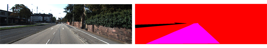
Fig. 1. An example of road pictures and the ground truth of the KITTI dataset.
Data Preprocessing: We need to ease the computation because the number of pixels per image could be huge (Since the resolution of images are about 375 * 1240. So there are more than 465,000 pixels per image), which would consume huge computation time if we apply complex methods on the data. Therefore, we firstly compute super-pixels using SLICO (zero parameter version of Simple Linear Iterative Clustering) for each image. After SLICO preprocessing, the average labels of super-pixels become float numbers in the range of [0, 1]. We define a threshold of 0.5 to decide the labels of super-pixels. If the prediction output is larger than 0.5, then it is determined as 1, which means it is road. Otherwise it is determined as 0, which means it is not road.
Model Selection: To compare the performance of different machine learning algorithms, we apply multiple learning models and construct their predication pipelines respectively. The models we have tried in our experiments are: K-NN, RBF-Kernel SVM, AdaBoost, RandomForest, Bagging, and Gaussian Naive Bayes.
Metrics: Since our objective is to investigate the performance of different machine learning techniques, we need to determine a evaluation metrics at the beginning. We use Score (Accuracy) as the major metrics.
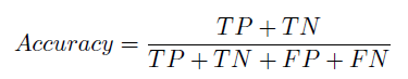
Where TP stands for True Positive, TN stands for True Negative, FP stands for False Positive and FN stands for False Negative. We evaluate the results both on super-pixel level and on pixel level for most of experiments.
Determine SLICO's Parameter: Since the road should always be continuous and has no isolated super pixels, using super-pixels for preprocessing to ease the computation will not affect the classification result too much. However, losses must be taken into consideration because of imperfect super-pixel segmentation. In SLICO preprocessing step, the major parameter for deciding the final outcome of segmentation is the number of super-pixels in each picture. After experimenting with a couple of different number of segments, we obtain the result that 1000 is a proper number of super-pixels, so we take 1000 as the parameter of our SLICO segmentation process.
Feature Selection: The selection of features need to be done before using classifiers to deal with road detection task. Since super-pixels are formed by aggregating single pixels, the most straightforward way seems to be taking the average RGB values of a super-pixel as its features. However, in fact, pixels have more information than just RGB values. For example, the location of a pixel can be very important when determining whether the pixel is road or not. Therefore, we add location information, which are average x, and y coordinates, into features. Furthermore, the size of each super-pixel could also provide useful information because each super-pixel consists of a number of single pixels. Therefore, we add super-pixel size into features.
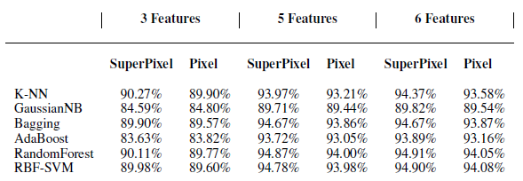
Fig. 2. Comparison of performance using Different Number of Features.
Since roads should always be continuous, it is reasonable to take the influence of the labels of a pixel’s neighbors into consideration when determining its own label. If its neighbors are already classified as road, then this pixel has a very high probability to be road as well. Thus, we use Pairwise CRF on a general graph. Pairwise potentials the same for all edges, are symmetric by default, which leads to n classes parameters for unary potentials. We implement GraphCRF on three different classifiers: Gaussian Naive Bayes, RandomForest and K-NN.

Fig. 3. The prediction result of K-NN before (left) and after (right) CRF.
We combine the prediction result with the original pictures, to demonstrate the performance of different machine learning techniques. Here is an example of the comparison result.
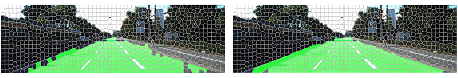
Fig. 4. The prediction result of K-NN before (left) and after (right) CRF.