Lab 9: Disease Propagation
This lab is part of Assignment 5. You are to complete the exercises here before arriving in lab on Monday/Tuesday. In lab, you and your partner will demonstrate your code to your TA, and get feedback. Your revised code is due on April 10 at noon.
In this assignment, we will be modeling how sexually transmitted infections propagate through populations. In epidemiology, the study of disease distribution, it is often useful to think of sexually active people as a graph. (Indeed, Wikipedia notes that "In a surprising result, mathematical models predict that the sexual network graph for the human race appears to have a single giant component that indirectly links almost all people who have had more than one sexual partner, and a great many of those who have had only one sexual partner (if their one sexual partner was themselves part of the giant component). Most people who are not part of the giant component are either virgins, or couples who have never had sex with anyone except each other.") Indeed, one such model of high school students found more than a quarter of the school was connected!
As always, your code must comply with the CS 190 Style Specifications, and work on the ECF machines. The marking scheme for Assignment 5 is available here.
Part Zero: Setup
Like the last assignment, you'll be submitting code via SVN.
You will need a partner for this assignment (which includes labs 9 and 10). Your partner must be from the same lab group as yourself. You may work with the same person you did for Assignment 4 provided they are in your lab group.
Like the last assignment, you and your partner will have to create a group on MarkUs so you may checkout the SVN repository for this assignment.
Part 1: Printing a Population
Worth knowing upfront: Unlike previous assignments, in this assignment, you will be marked for your code's efficiency. Keep this in mind when designing your code. You will also need to make your own Makefile for this assignment, which is to be handed in.
In lab, your TAs will be checking the correctness of at least two of the methods in this lab. The efficiency will be marked in the automarking phase. Your TAs will check whether you have run gprof on your code (Part Three) but will not mark you on the values that gprof gives you.
- Begin by downloading the files disease_model.h, disease_model.c, and
test_printing.c. Download the population files tiny_population.txt,
small_population.txt,
medium_population.txt,
large_population.txt,
and huge_population.txt.
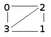
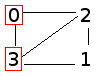
These files contain pairs of individuals (by ID number) who have had sex. Note that it will list all connections in the graph (e.g. 0, 2 and 2, 0). Starting with tiny_population, we have:
0, 2
0, 3
1, 2
1, 3
2, 0
2, 1
2, 3
3, 0
3, 2
3, 1
This indicates that person #0 has had sex with persons #2 and #3, and so on. The graph looks like this:
Similarly, small_population looks like:
And medium_population looks like:
- Begin implementing the functions in the file named disease_model.c, which reads in the contents of a population
file (given a filename), and loads it into a graph using a method read_file. You will also have to create and submit a Makefile for this assignment. When you compile test_printing with your Makefile, call the executable printing.
For the model, you will need to make a struct graph to store the graph in (as either an adjacency matrix or list). You will also need to make a struct person to represent the nodes in the graph. The Person structure should contain (you may extend it as you proceed through the assignment):
- If using an adjacency list: Connections to its sexual partners. You can store the
graph as either an adjacency matrix or a list (if using an adjacency matrix then the matrix would be stored in your struct graph instead.)
- An id number (integer); for tiny_population this would be 0-3.
- A disease status (char). "S" means the Person is susceptible to
the disease, "I" means the person has contracted the disease
and is infectious, and "V" means the person has been
vaccinated against the disease and cannot contract or share
the disease. People should begin with the status
"S". (We will not be using the V state in this lab, but it will be used in lab 10.)
- (Additional fields may be added for your implementation. For example, later on, such as in lab 10, you may want to add a field indicating how long a person has been infected for.)
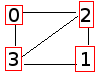
To summarize the graph, you will need to make a method print_stats which prints out how many people are in what condition. It must have the format like so:
STATS: S 100%, I 0%, V 0%; n = 4.
You will also need to make a method which prints the graph, print_graph, with its connections and the status of the person. It should also include statistics of how many people have status S, I, and V. It will look like (1 indicates a connection; 0 means no connection):
0,1,2,3 status
0 0,0,1,1 S
1 0,0,1,1 S
2 1,1,0,1 S
3 1,1,1,0 S
===============
STATS: S 100%, I 0%, V 0%; n = 4.
If a person is infected, it should also indicate how long they have been infected for. (See test_printing.txt for examples.) You should also create a method, remove_all that will free all the memory in a graph (and its associated persons).
- If using an adjacency list: Connections to its sexual partners. You can store the
graph as either an adjacency matrix or a list (if using an adjacency matrix then the matrix would be stored in your struct graph instead.)
Important! To test that your output matches my solution, you need to now download the file test_printing.txt and compare it to your own input. Assuming your executable is named printing, the steps to take are:
wget http://www.cs.toronto.edu/~patitsas/cs190/code/test_printing.txt
./printing > my_printing_output.txt
diff -s my_printing_output.txt test_printing.txt
The > operation on the command-line puts the output of your executable into the listed file (my_printing_output.txt). You can do this with any command in the terminal. The diff command gives you the difference between two files. If there are differences, it tells you what they are. With the -s flag present, it will tell you if the files are identical (without the -s, it will print nothing if given identical files).Your goal is to have no differences with my output.
Part Two: Infecting a Population (A Herpes Model)
- At this point, you should download test_infections.c which will give you more test cases to work with. Name its associated executable infections.
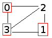
Now, create a method, seed_graph(int person), which seeds the disease in the population by giving a single person the disease. That person's status should now become I. The graph should, after calling seed_graph(0), would look like:

0,1,2,3 status
0 0,0,1,1 I (0)
1 0,0,1,1 S
2 1,1,0,1 S
3 1,1,1,0 S
===============
STATS: S 75%, I 25%, V 0%; n = 4.
-
Next, we will propagate the disease for one time step. Create
a method, propagate_once, which takes the graph as a
parameter. It also takes in a chance of transmission, that for now will always be 100%.
In this specific simulation, a person with status I has a 100% chance of infecting all their partners in one time step. (For this simulation, all partners are assumed to be current partners.) So, after calling this method once on our example, we should get:
 0,1,2,3 status
0 0,0,1,1 I (1)
1 0,0,1,1 S
2 1,1,0,1 I (0)
3 1,1,1,0 I (0)
===============
STATS: S 25%, I 75%, V 0%; n = 4.
If we call it a second time, we now get:
 0,1,2,3 status
0 0,0,1,1 I (2)
1 0,0,1,1 I (0)
2 1,1,0,1 I (1)
3 1,1,1,0 I (1)
===============
STATS: S 0%, I 100%, V 0%; n = 4.
- Create a method, propagate_n_times, which takes the
integer parameter n, and calls propagate_once n many times, and
prints out the statistics of each step. Its other parameters will be your graph, and the probability of transmission (which for now is always 100%.)
If we call propagate_n_times twice on our original graph, we should get the same result as what we have in step #2. Furthermore, since we have no way of simulating people getting better -- and people do not die -- this graph will not change any more.
Each time we propagate we will refer to as a time step in our simulation -- here, two time steps are all it takes for all of the members of tiny_population to be infected.
-
At this moment, we have a simulation of STIs like herpes, for
which there is no cure, but is not fatal. However, a person
infected with herpes does not have a 100% chance of infecting
their partners.
As such, let's now refine our propagate methods to take probability into account. The provided probability should be a double between 0 and 1 (inclusive). Let's say an infected person has a 50% (0.5) chance of infecting a given partner. The propagation now might look like:
We've used a standard seed in our test files to ensure everybody has the same "random numbers". Make sure you only call rand once in a given call to propagate_once, to keep your output consistent with mine. Use the test cases in test_infect.c to ensure your output is the same.
Similar to the last part, you now want to do these steps:
wget http://www.cs.toronto.edu/~patitsas/cs190/code/test_infections.txt
./infections > my_infection_output.txt
diff -s my_infection_output.txt test_infections.txt
Again, you want to ensure your output matches test_infection.txt, and that diff gives you no differences.
Part Three: Optimization
Unlike previous assignments, your code in this assignment will be marked for efficiency. To profile the efficiency of your code, you are to use gprof (You can read more about gprof here and here).
Download the file test_fast.c and compile it with the -pg flag to enable profiling.
Name the executable fast. Then run:
./fast > output.txt
This will output the results of the executable into the file output.txt. Then:
gprof fast > profile_result.txt
This will put the profiling results in profile_result.txt.
Compare your profile_result.txt to these two: slow_profile.txt and fast_profile.txt. Your helper methods may make the profiling look different. What is important is the total s/call column, which tells us how much time was spent calling a given method. Any time spent in helper methods will be included in this number.
We expect your total s/call for read_file, seed_graph and remove_all to be 0 seconds on remote.ecf.utoronto.ca
You'll note that slow_profile.txt and fast_profile.txt differ in the total s/call for propagate_n_times: 6.73 seconds vs. 3.11 seconds.
For one point in this assignment, you need your propagate_n_times to be faster or equal to 6.73 seconds; for a second point it needs to be faster or equal to 3.11 seconds. Both need to be timed on remote.ecf.utoronto.ca in order to be valid comparisons to my provided data. (The values will differ on other computers!) Enabling compiler optimization is acceptable (if not recommended), but probably not enough to get you under 3.11 seconds.
You are to hand in your profile_result.txt for this assignment.
You'll also want to check that your code is producing the correct output. You can do this as such:
wget http://www.cs.toronto.edu/~patitsas/cs190/code/slow_output.txt
diff -s output.txt slow_output.txt
If there are no differences between the files, and the "-s" is present, it will say that the files are identical.
Finally, ensure there are no memory leaks in any of your test files (test_printing.c, test_infections.c, test_fast.c) by running valgrind on these. We will be deducting marks in the automarking phase for any memory leaks and any memory errors reported by valgrind, as well as any compiler warnings (with -Wall enabled).
Waiting to Talk to Your TA?
Get started on Lab 10!