Deep Spectral Clustering Learning

Clustering is the task of grouping a set of examples so that similar examples are grouped into the same cluster while dissimilar examples are in different clusters. The quality of a clustering depends on two problem-dependent factors which are i) the chosen similarity metric and ii) the data representation. Supervised clustering approaches, which exploit labeled partitioned datasets have thus been proposed, for instance to learn a metric optimized to perform clustering. However, most of these approaches assume that the representation of the data is fixed and then learn an appropriate linear transformation. Some deep supervised clustering learning approaches have also been proposed. However, they rely on iterative methods to compute gradients resulting in high algorithmic complexity. In this paper, we propose a deep supervised clustering metric learning method that formulates a novel loss function. We derive a closed-form expression for the gradient that is efficient to compute: the complexity to compute the gradient is linear in the size of the training mini-batch and quadratic in the representation dimensionality. We further reveal how our approach can be seen as learning spectral clustering. Experiments on standard real-world datasets confirm state-of-the-art Recall@K performance.

Tensorflow 0.12 code

We follow the notations of the paper where F is the output representation matrix of the mini-batch and Y is the desired/ground truth assignment matrix. Our loss function can be written:

def supervised_clustering_loss(F,Y):
    diagy = tf.reduce_sum(Y,0)
    onesy = tf.ones(diagy.get_shape())
    J = tf.matmul(Y,tf.diag(tf.rsqrt(tf.select(tf.greater_equal(diagy,onesy),diagy,onesy))))
    [S,U,V] = tf.svd(F)
    Slength = tf.cast(tf.reduce_max(S.get_shape()), tf.float32)
    maxS = tf.fill(tf.shape(S),tf.scalar_mul(tf.scalar_mul(1e-15,tf.reduce_max(S)),Slength))
    ST = tf.select(tf.greater_equal(S,maxS),tf.div(tf.ones(S.get_shape()),S),tf.zeros(S.get_shape()))
    pinvF = tf.transpose(tf.matmul(U,tf.matmul(tf.diag(ST),V,False,True)))
    FJ = tf.matmul(pinvF,J)
    G = tf.matmul(tf.sub(tf.matmul(F,FJ),J),FJ,False,True)
    loss = tf.reduce_sum(tf.mul(tf.stop_gradient(G),F))
    return loss


We minimize this loss with the standard GradientDescentOptimizer.

You can also keep track of the value of the loss in Eq. (10) with the following loss:

   monitor_loss = - tf.reduce_sum(tf.mul(FJ,tf.matmul(F,J,True)))


The value of monitor_loss should be between 0 and -k. You can add k to make monitor_loss nonnegative. The lower the value, the better. Note that you should optimize loss with gradient descent, not monitor_loss which is only used to keep track of the loss value.

Matlab/Octave gradient code

The Matlab/Octave code in the supplementary material to verify the gradient is:

clear all;

n = 10;
d = 4;
rank_of_C = 7;

Y = rand(n,rank_of_C)*10;
C = Y * pinv(Y);

F = (rand(n,d)*10) - 5;
Real_gradient = 2*(eye(n) - F*pinv(F)) * C * pinv(F)';
epsilon = 10^-7;

Approximate_gradient = zeros(n,d);

for i=1:n
  for j=1:d
    E = zeros(n,d);
    E(i,j) = epsilon;

    X1 = F+E;
    X2 = F-E;

    Approximate_gradient(i,j) = (trace(X1 * pinv(X1) * C) - trace(X2 * pinv(X2) * C))/(2*epsilon);
  end
end


Real_gradient
Approximate_gradient

disp('Frobenius distance')
norm(Real_gradient-Approximate_gradient,'fro')


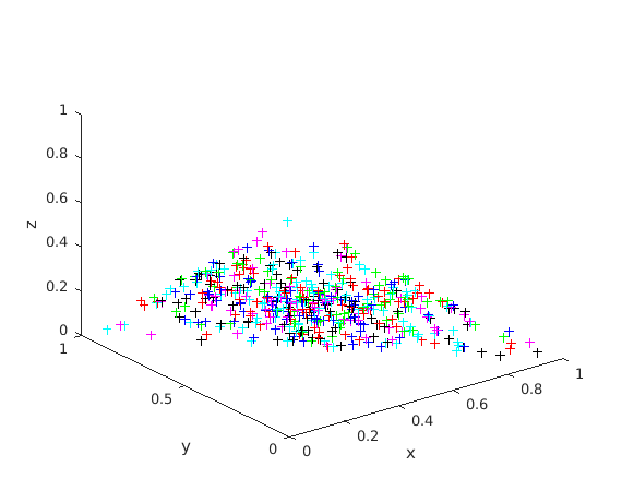
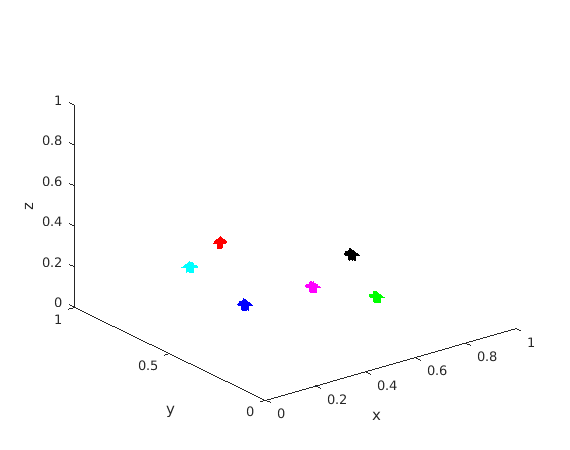
Visual demo in Matlab/Octave

We provide the code for a visual demo in Matlab/Octave where the examples are in a 3d-simplex. The examples are initialized randomly and belong to 6 desired clusters (1 color for each desired cluster): The representation of the examples is learned so that similar examples are grouped in the same cluster via projected gradient descent (the samples are projected onto the simplex at each iteration). After about 150 iterations of gradient descent, the representation of the examples looks like this: