Monitor without labels
No training set at deployment
Statistical guarantees
Method Overview
D3M (Disagreement-Driven Deterioration Monitoring) proceeds in three stages: Train, Calibrate, and Deploy.
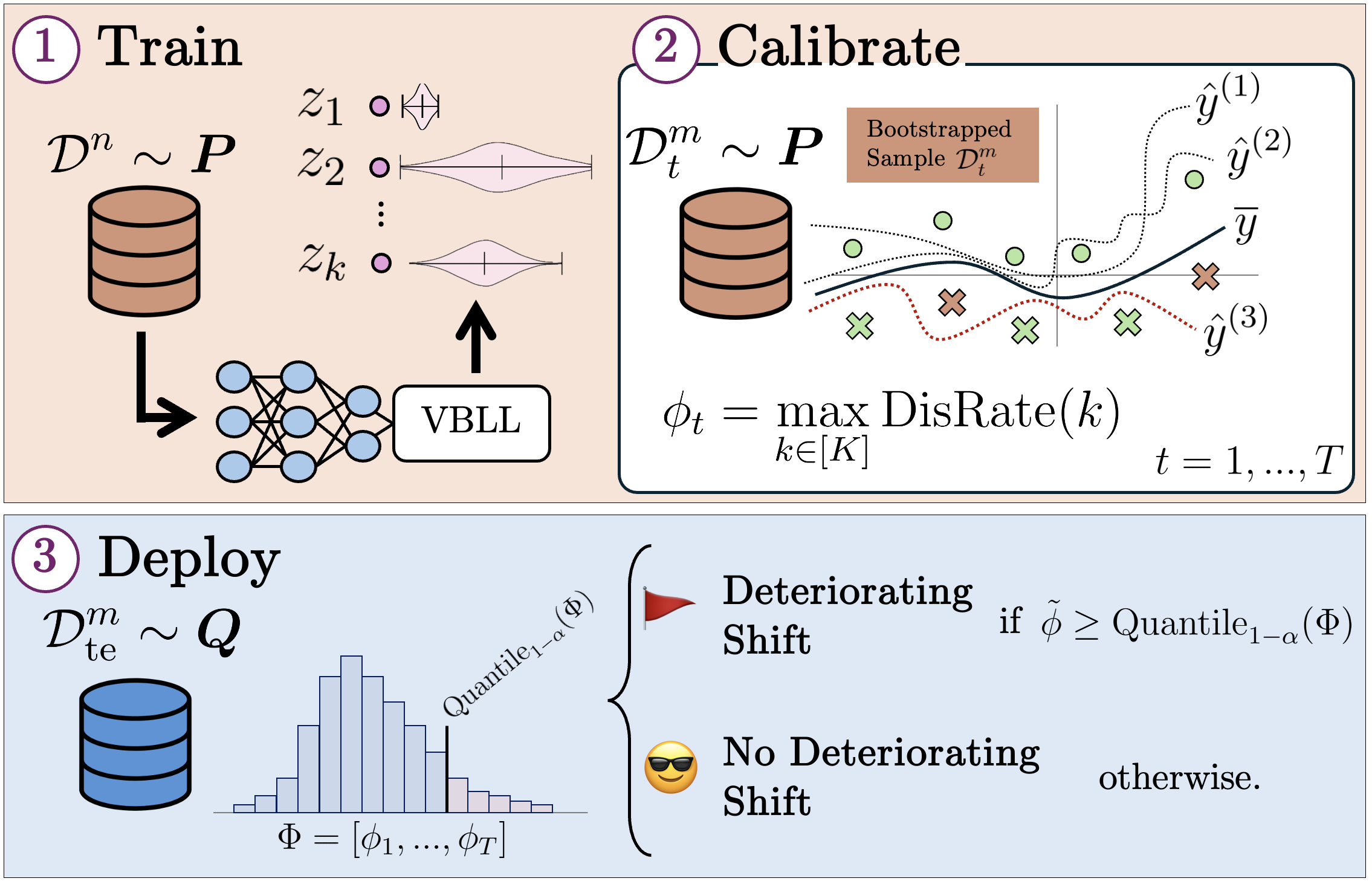
1. Train — Base model learning
A composition \(\operatorname{VBLL}_\theta \circ \operatorname{FE}_\theta\) of a neural feature extractor \( \operatorname{FE}_\theta : \mathcal{X} \to \mathbb{R}^d \) and a Variational Bayesian Last Layer (VBLL) \( \operatorname{VBLL}_\theta : \mathbb{R}^d \to \mathcal{P}(\mathbb{R}^C) \) is trained on supervised ID data \( \mathcal{D}^n \sim \mathbb{P}^n \) to produce posteriors over logits for \( C \) classes:
The base model defines the posterior predictive distribution (PPD):
Training maximizes the ELBO with Gaussian prior \( p(z) \):
2. Calibrate — ID Disagreement statistics
On held-out ID data, we repeatedly bootstrap \( \mathcal{D}^m_t = \{x_i\}_{i=1}^m \sim \mathbb{P}^m \), and compute maximum disagreement rates \( \phi_t \). Base model pseudo-labels are obtained as:
We draw \( K \) posterior samples, apply temperature scaling, and sample labels:
The disagreement rate for sample \( k \) is:
and the maximum disagreement rate for round \( t \):
The collection of all ID disagreements forms \( \Phi = \{\phi_t : t \in [T]\} \).
3. Deploy — Deterioration monitoring
At deployment, we collect unlabeled batches \( \mathcal{D}^m_{\text{te}} \sim \mathbb{Q}^m \) and compute the same statistic \( \tilde{\phi} \). The system raises an alert if:
ensuring a FPR bounded by \( \alpha \) under ID conditions.
Theory
For a formal theoretical analysis and sample complexities to guarantee low FPR and high TPR with high probability, please visit Appendix A in our paper!
Why does this work?
- We need a computable quantity \(\phi\) independent of labels, whose value statistically differs ID and OOD if and only if model deterioration occurs.
- It turns out, model disagreement rate fits exactly this description if the deterioration is due to a shift in covariates!
- Thus, our method estimates an empirical distribution of ID disagreement rates \(\Phi\). Deterioration detection simply regresses to determining whether a sample's model disagreement rate could've come from \(\Phi\)!
What is model disagreement?
Assume among a family \(\mathcal{H}\), an ERM algorithm on ID training samples \(\mathcal{D}^n\) selects hypothesis \(f\). Among other competing hypotheses \(h\) explaining \(\mathcal{D}^n\), the ID model disagreement rate is the disagreement rate of the maximally disagreeing hypothesis \(h\) with respect to \(f\) on a held-out ID validation batch.
The search for a maximally disagreeing hypothesis is difficult. We turn this optimization problem into a sampling problem by sampling candidate hypotheses from a Bayesian model, and taking the maximally disagreeing hypothesis.
We thus chart an empirical distribution of approximate disagreement rates for random bootstraps of a held-out ID validation set to obtain a robust statistical quantification of the ID disagreement rate.
Implementation details
The composition \(\operatorname{VBLL}_\theta \circ \operatorname{FE}_\theta\) is trained end-to-end on ID data of size \( n \) by maximizing the ELBO. For calibration, across rounds \( t \in [T] \), we sample datasets \( \mathcal{D}^m_t \) of size \( m \ll n \) (with replacement) from a large held-out ID validation set. Each \( \mathcal{D}^m_t \) is processed in a single forward pass, producing \( m \) independent \( C \)-dimensional Gaussian posteriors:
$$q_\theta(z_i \mid x_i) ≔ \mathcal{N}(z_i \mid \mu_\theta(x_i), \operatorname{diag}(\sigma_\theta^2(x_i)))$$
For each posterior, we draw \( 2K \) samples—\( K \) for Monte Carlo estimation of the mean model, and \( K \) for maximum-disagreement computations. We keep the sampling temperature \( \tau \), the dataset size \( m \), and the number of posterior samples \( K \) as tunable hyperparameters. Crucially, these must be identical between the computation of \( \Phi \) and the subsequent deployment-time monitoring test, where the exact same procedure is applied on a deployment sample \( \mathcal{D}^m_{\textbf{te}} \).
Monitoring large models
The flexibility of D3M lies in the broad selection of \(\operatorname{FE}_\theta\). Vision language model features may be used to monitor vision classification tasks, while language model bases such as BERT may be used as feature extractors for text classification tasks.
Of course, as stated, this does not work for any classification model based on in-context prompting due to D3M's reliance on \(\operatorname{VBLL}_\theta\), and is work in progress.
Results
We summarize performance on both classical benchmarks and real-world GEMINI clinical data. Full quantitative tables and visualizations are available in the paper.
Classical Benchmarks
D3M demonstrates strong TPR across a diverse set of datasets — UCI Heart Disease, CIFAR-10/10.1, and Camelyon-17 — while maintaining controlled FPR under ID calibration.
| UCI Heart Disease | CIFAR 10.1 | Camelyon 17 | |||||||
|---|---|---|---|---|---|---|---|---|---|
| 10 | 20 | 50 | 10 | 20 | 50 | 10 | 20 | 50 | |
| BBSD | .13±.03 | .22±.04 | .46±.05 | .07±.03 | .05±.02 | .12±.03 | .16±.04 | .38±.05 | .87±.03 |
| Rel. Mahalanobis | .11±.03 | .36±.05 | .66±.05 | .05±.02 | .03±.03 | .04±.02 | .16±.04 | .40±.05 | .89±.03 |
| Deep Ensemble | .13±.03 | .32±.05 | .64±.05 | .33±.05 | .52±.05 | .68±.05 | .14±.03 | .26±.04 | .82±.04 |
| CTST | .15±.04 | .51±.05 | .98±.01 | .03±.02 | .04±.02 | .04±.02 | .11±.03 | .59±.05 | .59±.05 |
| MMD-D | .09±.03 | .12±.03 | .27±.04 | .24±.04 | .10±.03 | .05±.02 | .42±.05 | .62±.05 | .69±.05 |
| H-Div | .15±.04 | .26±.04 | .37±.05 | .02±.01 | .05±.02 | .04±.02 | .03±.02 | .07±.03 | .23±.04 |
| Detectron | .24±.04 | .57±.05 | .82±.04 | .37±.05 | .54±.05 | .83±.04 | .97±.02 | 1.0±.00 | .96±.02 |
| D3M (Ours) | .38±.19 | .25±.28 | .69±.33 | .40±.10 | .45±.10 | .74±.12 | .89±.20 | .93±.05 | .99±.02 |
Table 1. True positive rates (TPR) comparison across datasets and query sizes. As models experience deterioration, higher TPR indicates better detection performance. Bold values denote column best; results are averaged over 10 independent seeds. D3M results are averaged across runs achieving ID FPR below \(\alpha\).
Results on GEMINI
Results illustrating D3M’s deployment on GEMINI, an EHR dataset with tabular engineered features. The task is 14-day mortality prediction.
Non-deteriorating temporal shift:
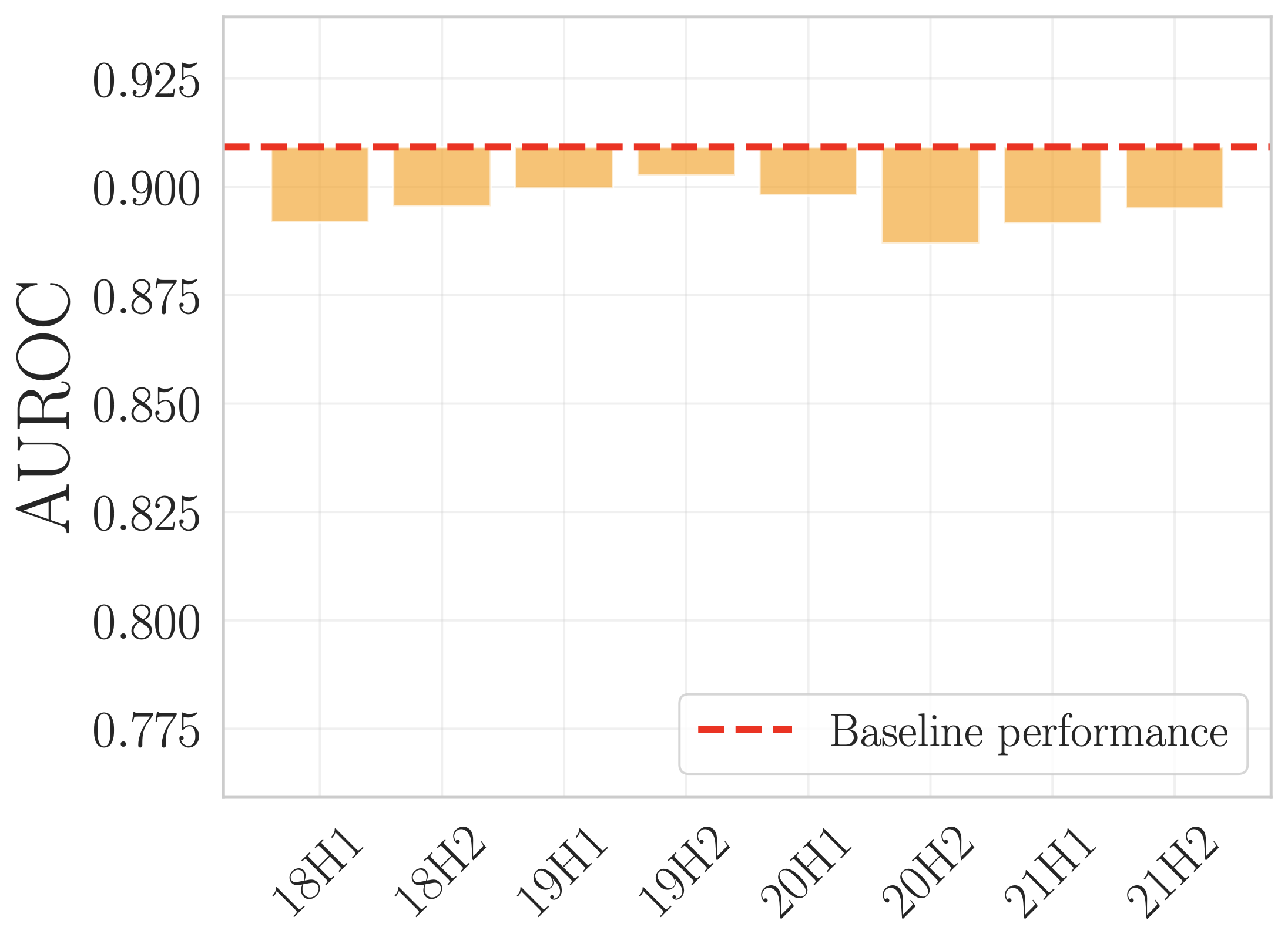
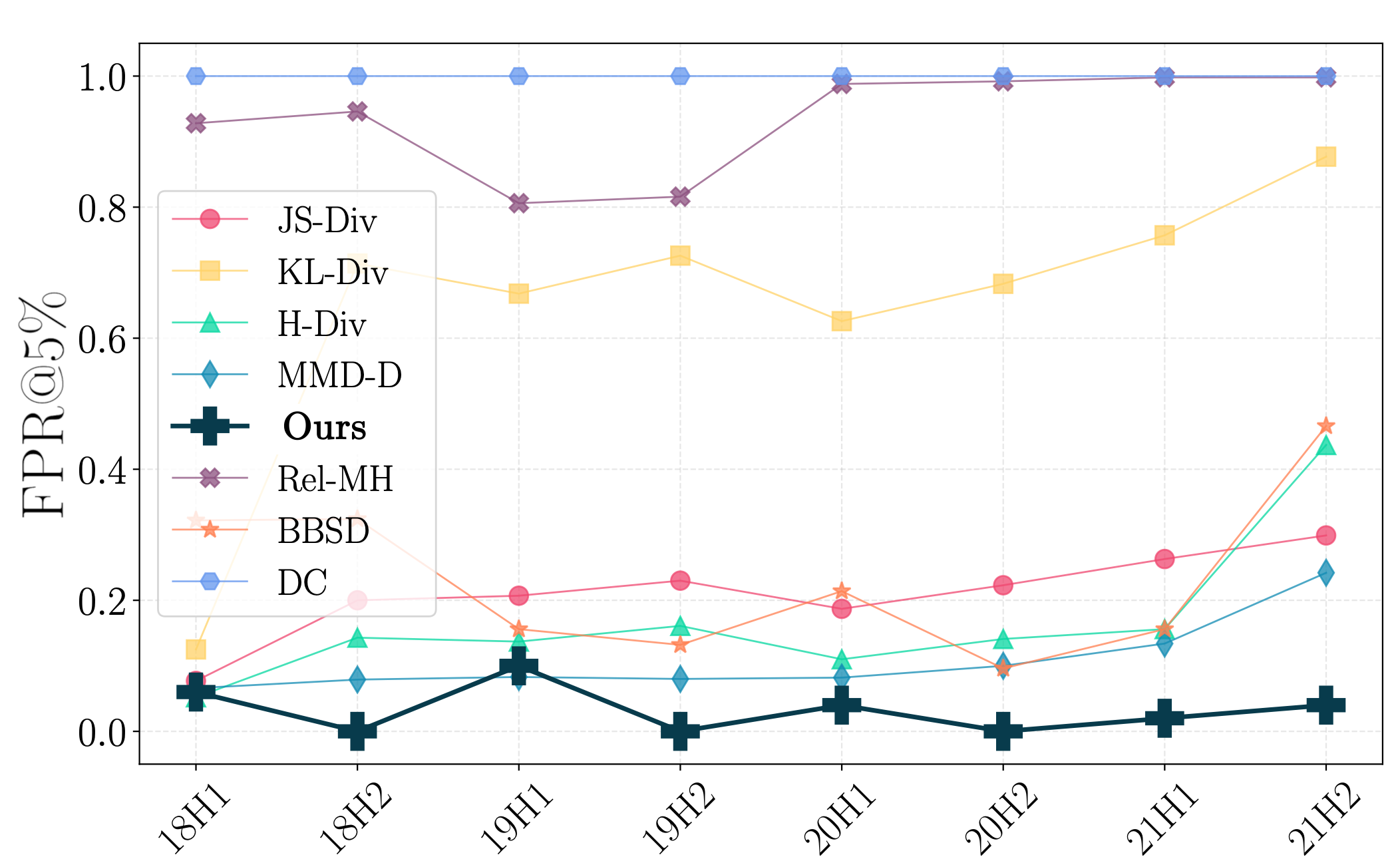
(Left) Performance of the base model over half-years since 2017. Little drop in performance is observed, the natural temporal shift is thus non-deteriorating. (Right) Indeed, D3M does not pick up on longitudinal distribution shifts. We know these shifts exist since distance-based baselines (JS-Div, KL-Div, Relative Mahalanobis) heavily flag these changes.
Manufactured deteriorating shift:
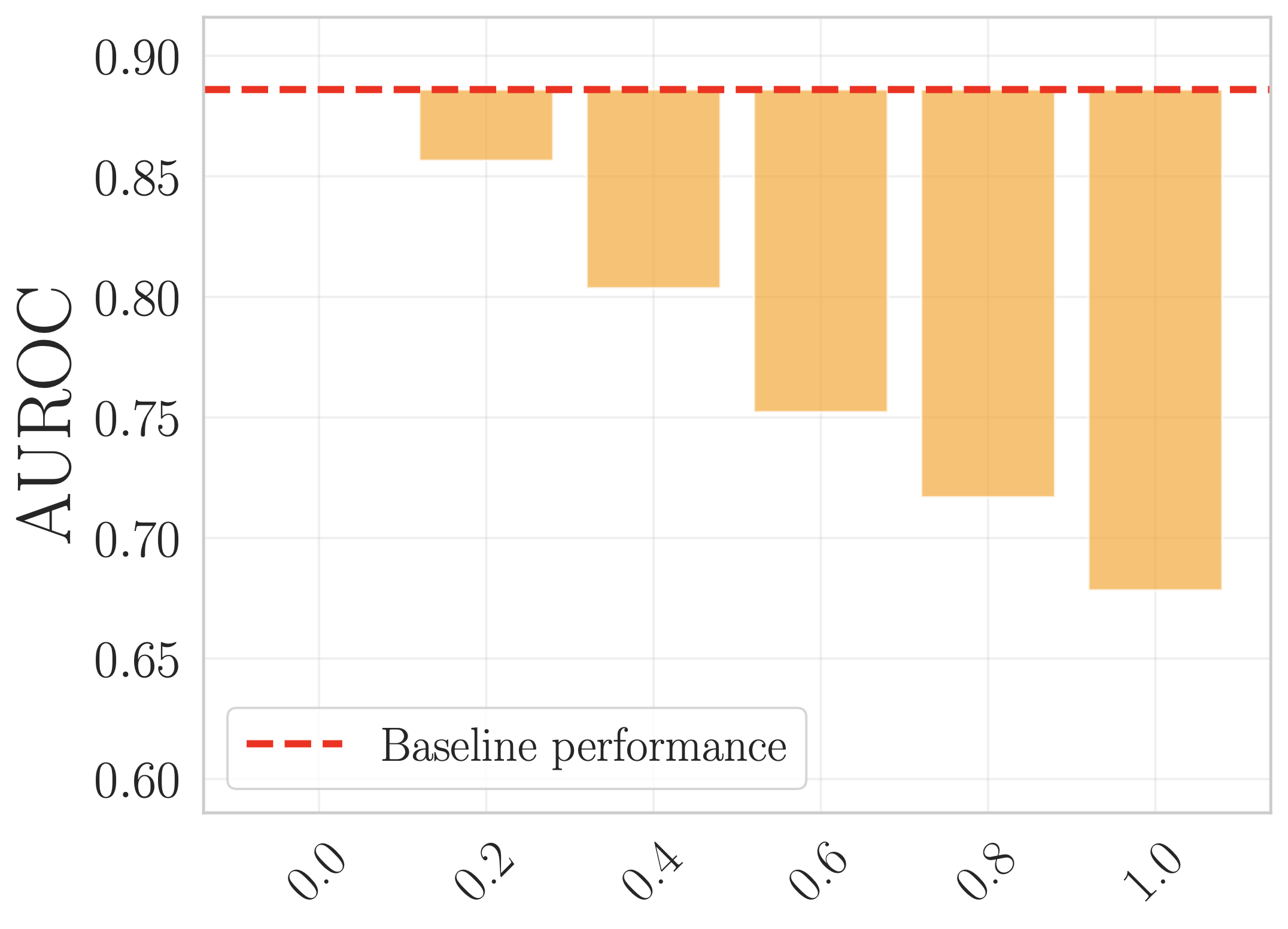
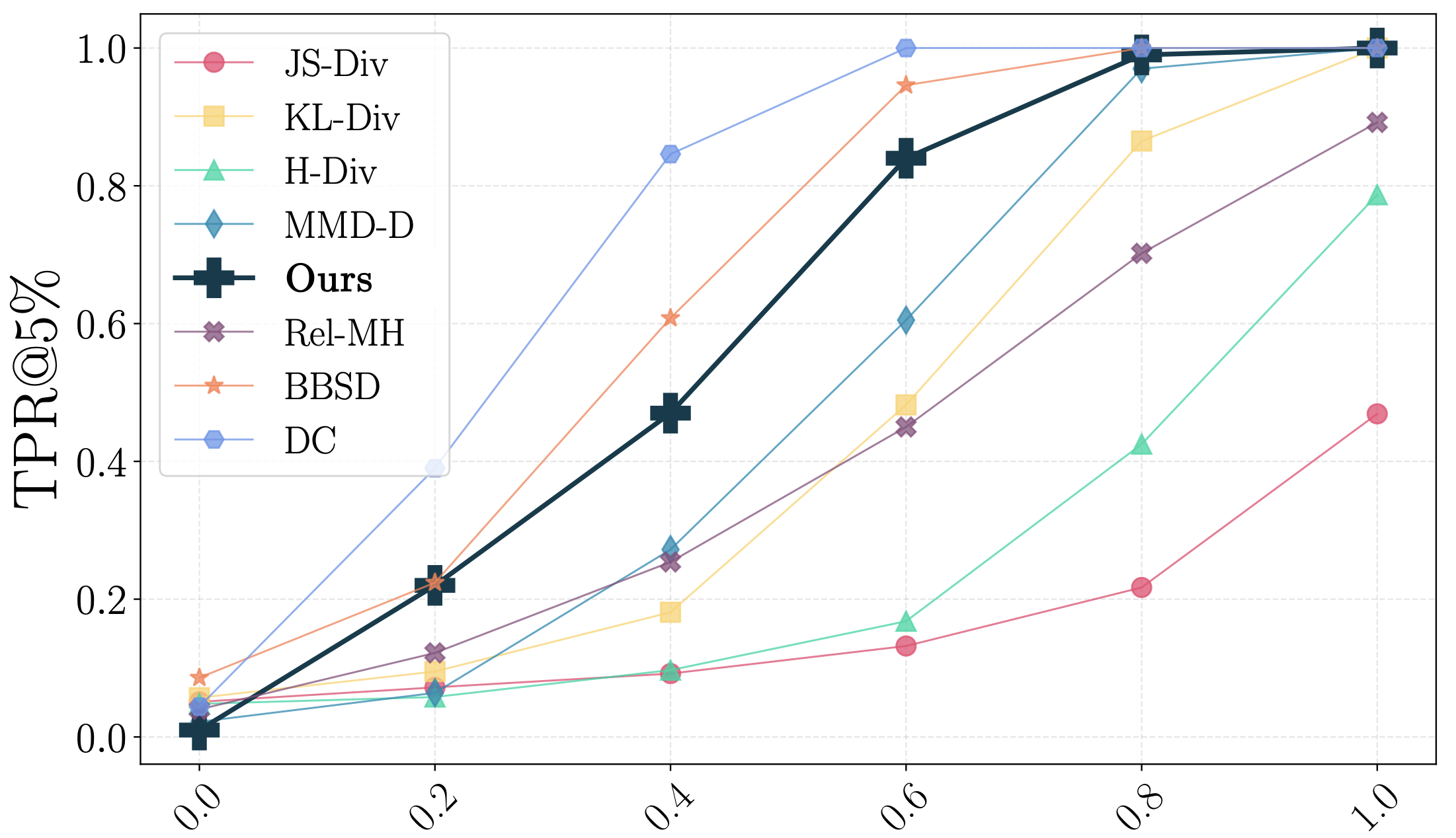
(Left) The base model is trained on patients between 18-52 years of age. Then, the model is deployed on mixtures of test data mixed at different ratios with patients above 85 years old to induce an artificial distribution shift. Indeed, model deterioration is observed. (Right) D3M's TPR grows stronger as more OOD data is mixed into the deployment test sample.
Authors
The team behind D3M: Disagreement-Driven Deterioration Monitoring.

Viet Nguyen†
University of Toronto

Changjian Shui†
University of Ottawa

Vijay Giri
University of Pennsylvania

Siddharth Arya
University of Toronto

Amol Verma
Unity Health Toronto

Fahad Razak
Unity Health Toronto

Rahul G. Krishnan
University of Toronto
BibTeX tag
If you find this work useful in your research, please cite:
@inproceedings{nguyen2025disagreement,
  title={Reliably detecting model failures in deployment without labels},
  author={Nguyen, Viet and Shui, Changjian and Giri, Vijay and Arya, Siddharth and Verma, Amol and Razak, Fahad and Krishnan, Rahul G},
  booktitle = {Proceedings of the Conference on Neural Information Processing Systems (NeurIPS)},
  year={2025},
}