Delayed and Focused Profiling

Since neural network libraries may include tuning operations at the start of training, to obtain a representative sample of the training process, we wait multiple iterations before turning on profiling. With python, we use the numba library to control when profiling samples are taken.

import numba.cuda as cuda

We call cuda.profile_start() to begin the profiling, and cuda.profile_stop() to end profiling. Since generated profile files can become large and each training iteration follows the same computation logic, the profiling period is usually chosen to be only a small number of iterations. Moreover, we carefully choose a period that includes only training computations, without validation. After cuda.profile_stop() is hit, the training process can be safely killed with Ctrl+c. The .nvvp file exported by the --export-profile option can be viewed by NVidia Visual Profiler for further analysis.

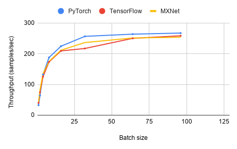
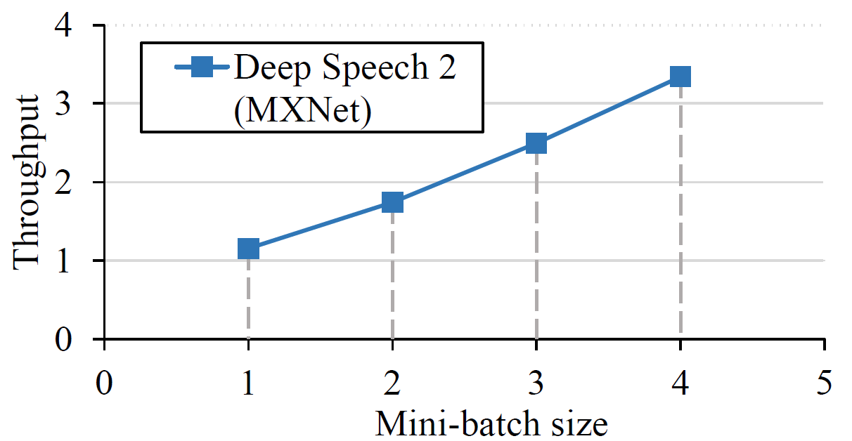
Throughput

Throughput measures the number of training cases or samples, where applicable, that are processed per second during training. Most benchmarks already have throughput statistics output in training logs without additional work. For Deep Speech 2, which has no training throughput numbers logged directly, we measure the sum of all data samples between two time stamps in the training logs. As the lengths of the data samples vary a lot, we use the total length of data samples instead of a simple count to measure training throughput with Deep Speech 2.

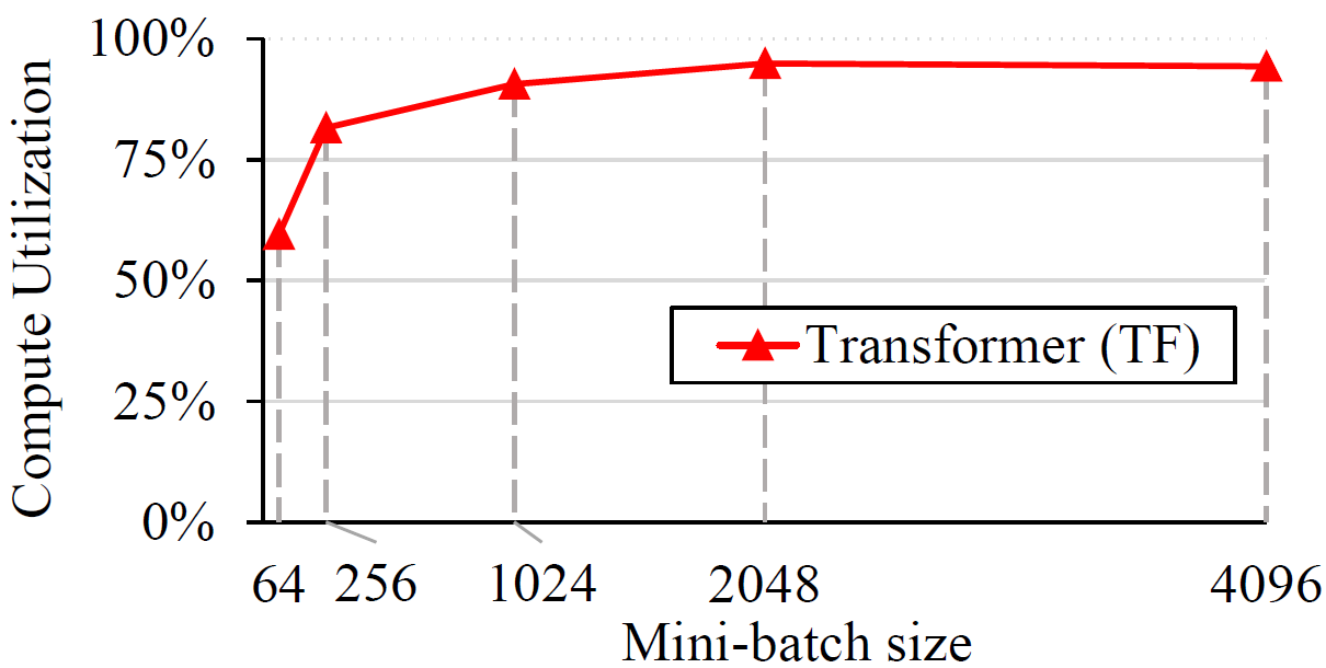
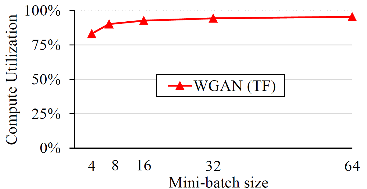
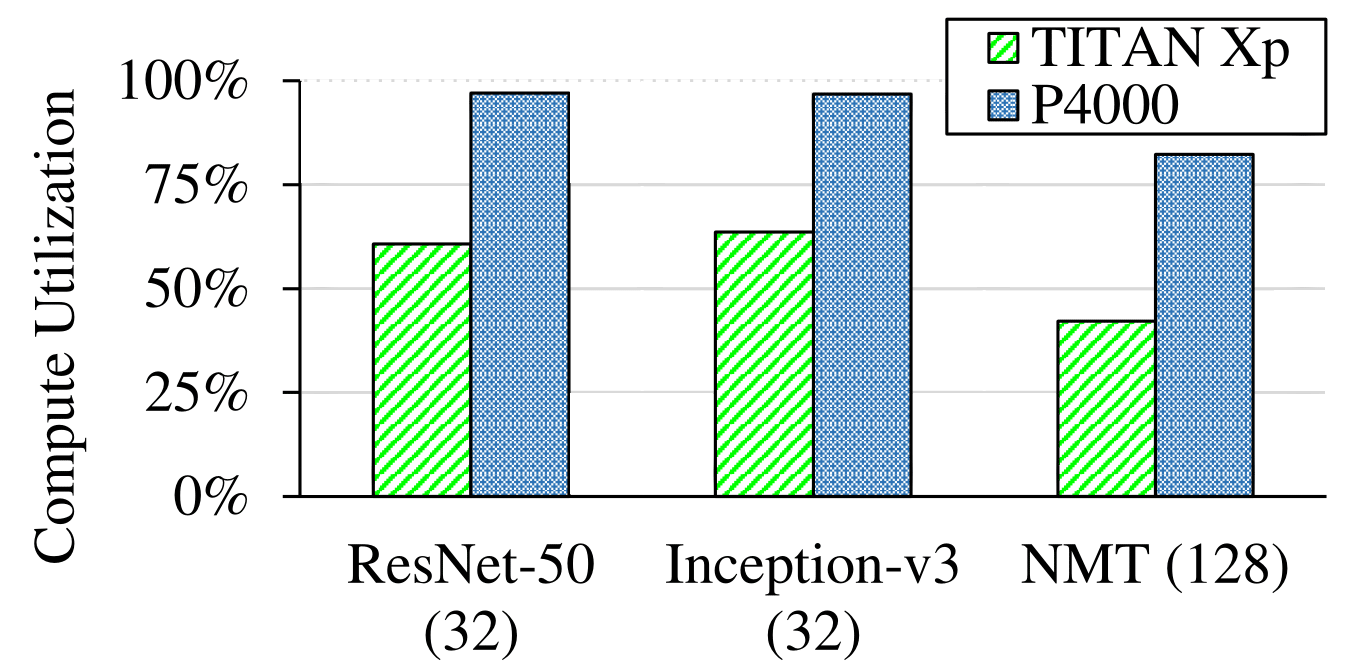
Compute Utilization

GPU compute utilization measures the relative amount of time that the GPU spends actively running kernels. NVidia Visual Profiler provides this information directly, but the profiling overhead time should be excluded from that number.

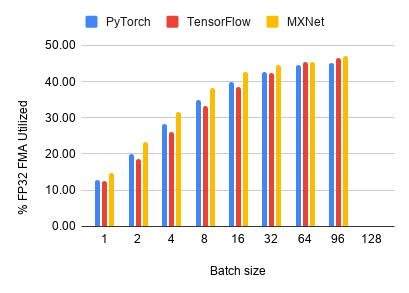
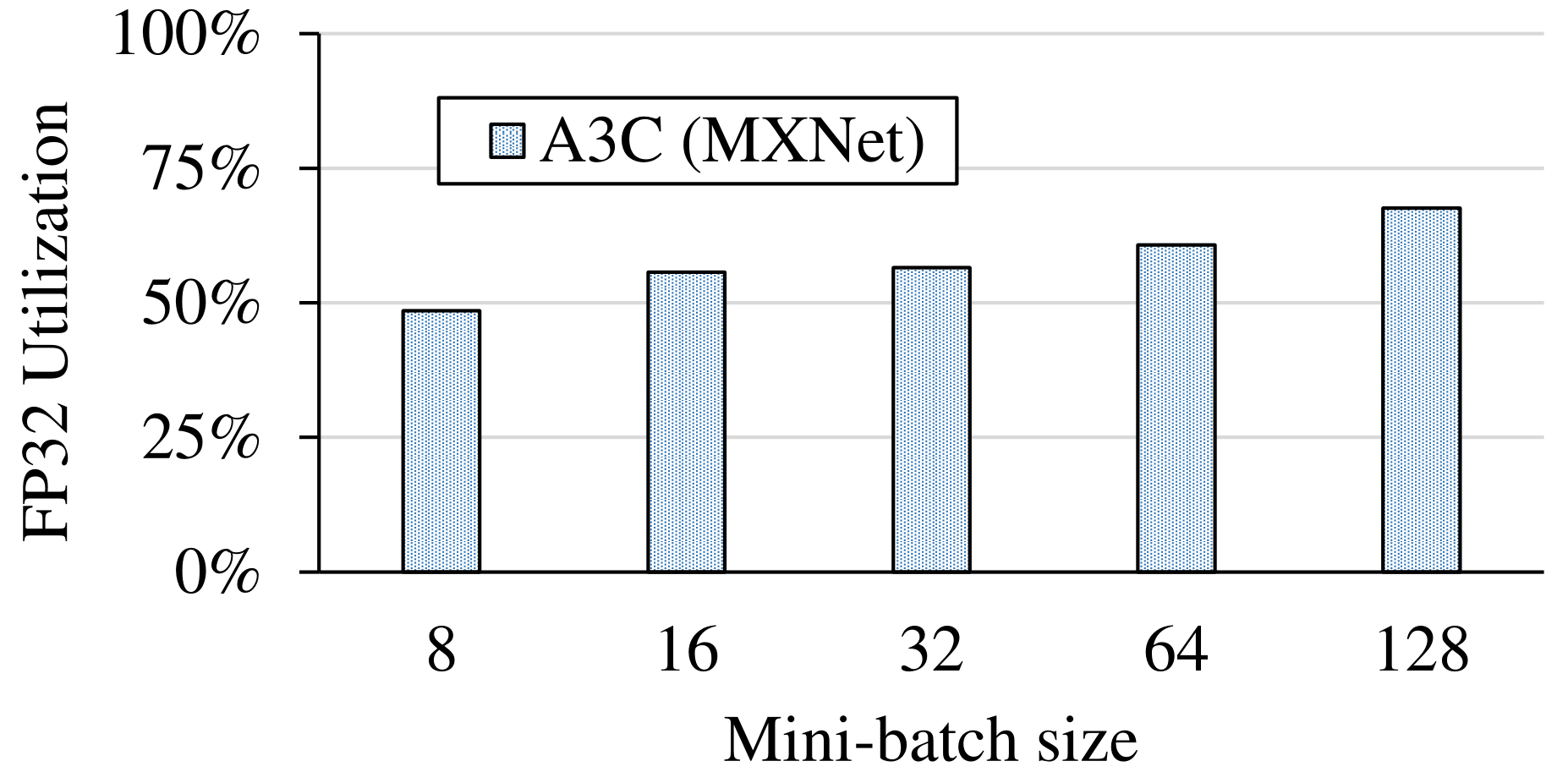
Floating-Point Utilization

GPU floating point utilization quantifies how busy the GPU's floating-point compute units are during training. This is informative since floating-point arithmetic comprises the majority of computation in all benchmarks. This is reported by the profiler when run with the --metrics single_precision_fu_utilization option as above. The profiler generates the FP32 utilization for each individual kernel. We calculate a weighted sum over all kernels for the overall FP32 utilization of the training. We can also determine which kernels are long but with low utilization. Such kernels are good targets for optimization.

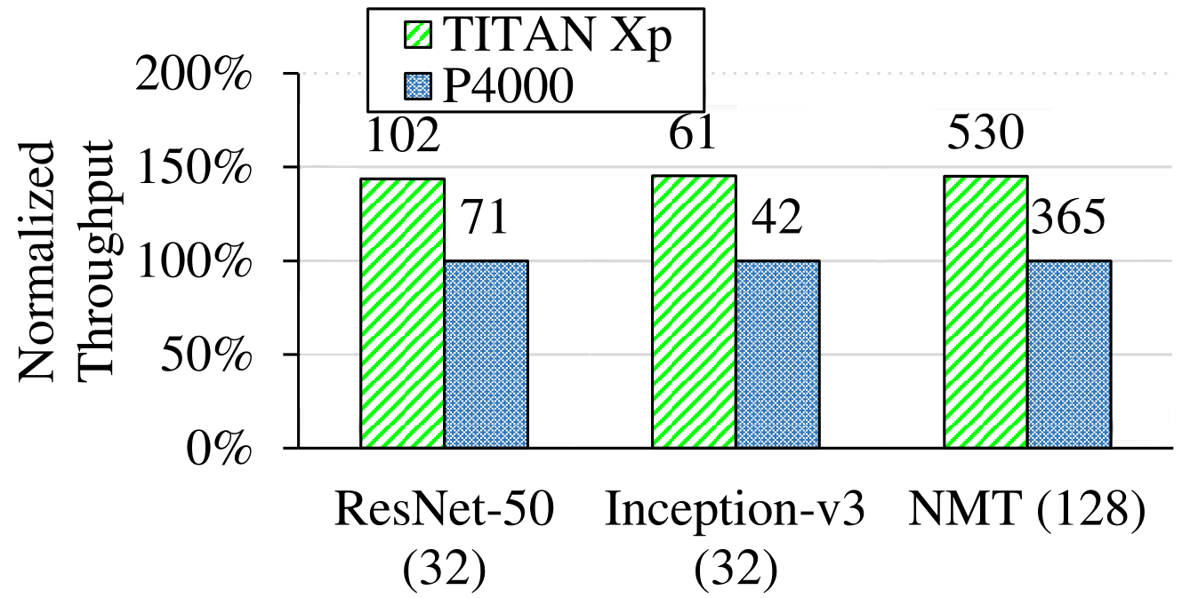
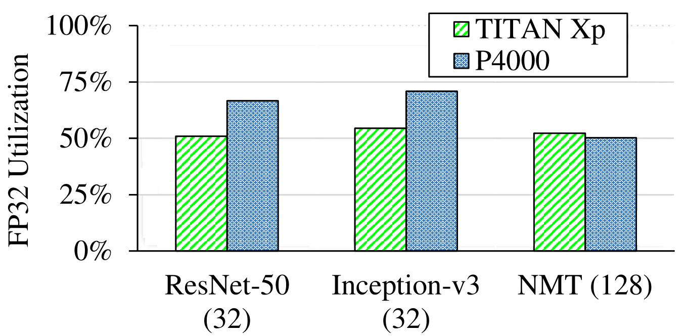
Hardware Sensitivity

We studied how the performance of DNN training is affected by the hardware used. We used TitanXp for comparison against Quadro P4000. Detailed hardware specifications of these two types GPU are shown following:

	# of Multi-processors	Core count	Max Clock Rate (MHz)	Memory Size (GB)	LLC Size (MB)	Memory Bus Type	Memory BW (GB/s)	Bus Interface	Memory Speed (MHz)
TitanXp	30	3840	1582	12	3	GDDR5X	547.6	PCIe 3.0	5705
P4000	14	1792	1480	8	2	GDDR5	243	PCIe 3.0	3802

We compare the training throughput, GPU utilization and FP32 utilization. The results show that although the more advanced GPU (Titan Xp) delivers better training throughput, its compute resources are still under-utilized.

Distributed Training

Training large DNNs can be done faster when multiple GPUs and/or multiple machines are used. This is usually achieved by using data parallelism, where mini-batches are split among individual GPUs and the results are then merged. We studied how the scalability is affected by the network bandwidth. We tested the training of ResNet-50 on MXNet on both multi-GPU and multi-machine environments. Our prilimary results show that the bandwidth of 1 Gb/s ethernet will greatly lower the overall training performance, and that the bandwidth of 100 Gb/s infiniband is sufficient for delivering good scalability in a multi-machine environment.


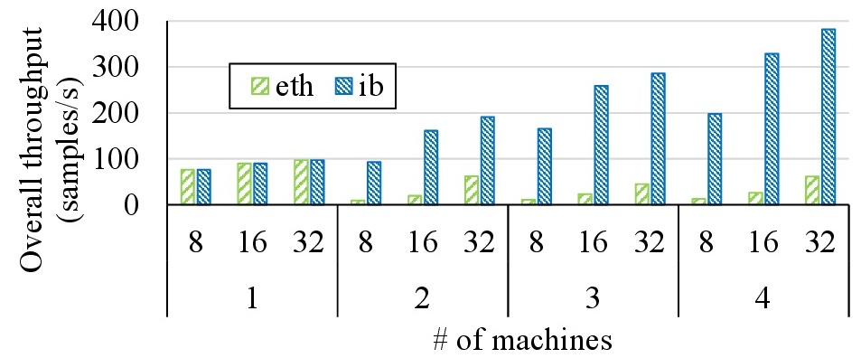
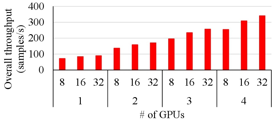
The first level of the x-axis shows the per-machine mini-batch size, and the second level of the x-axis shows the number of machines. In the case where multiple GPUs located in the same machine, all GPUs are connected with the host through a 6 GB/s PCIe bus. It is able to deliver high scalability, but slightly lower throughput.