Transpose Convolutions and Autoencoders
In our discussions of convolutional networks, we always started with an image, then reduced the "resolution" of the image until we made an image-level prediction. Specifically, we focused on image level classification problems: is the image of a cat or a dog? Which of the 10 digits does this image represent? We always went from a large image, to a lower-dimensional representation of the image.
Some tasks require us to go in the opposite direction. For example, we may wish to make pixel-wise predictions about the content of each pixel in an image. Is this pixel part of the foreground or the background? Is this pixel a part of a car or a pedestrian? Problems that require us to label each pixel is called a pixel-wise prediction problem. These problems require us to produce an high-resolution "image" from a low-dimensional representation of its contents.
A similar task is the task of generating an image given a low-dimensional embedding of the image. For example, we may wish to produce a neural network model that generates images of hand-written digits not in the MNIST data set. A neural network model that learns to generate new examples of data is called a generative model.
In both cases, we need a way to increase the resolution of our hidden units. We need something akin to convolution, but that goes in the opposite direction. We will use something called a transpose convolution. Transpose convolutions were first called deconvolutions, since it is the ``inverse'' of a convolution operation. However, the terminology was confusing since it has nothing to do with the mathematical notion of deconvolution.
import torch
import torch.nn as nn
import torch.nn.functional as F
import torch.optim as optim
import matplotlib.pyplot as plt
from torchvision import datasets, transforms

mnist_data = datasets.MNIST('data', train=True, download=True, transform=transforms.ToTensor())
mnist_data = list(mnist_data)[:4096]
Convolution Transpose
We can make a tranpose convolution layer in PyTorch like this:
convt = nn.ConvTranspose2d(in_channels=16,
                           out_channels=8,
                           kernel_size=5)
Here's an example of this convolution transpose operation in action:
x = torch.randn(32, 16, 64, 64)
y = convt(x)
y.shape
Notice that the width and height of y is 68x68, because the kernel_size is 5
and we have not added any padding. You can verify that if we start with a tensor
with resolution 68x68 and applied a 5x5 convolution, we would end up with
a tensor with resolution 64x64.
conv = nn.Conv2d(in_channels=8,
                 out_channels=16,
                 kernel_size=5)
y = torch.randn(32, 8, 68, 68)
x = conv(y)
x.shape
As before, we can add a padding to our convolution transpose, just like we added padding to our convolution operations:
convt = nn.ConvTranspose2d(in_channels=16,
                           out_channels=8,
                           kernel_size=5,
                           padding=2)
x = torch.randn(32, 16, 64, 64)
y = convt(x)
y.shape
More interestingly, we can add a stride to the convolution to increase our resolution!
convt = nn.ConvTranspose2d(in_channels=16,
                           out_channels=8,
                           kernel_size=5,
                           stride=2,
                           output_padding=1, # needed because stride=2
                           padding=2)
x = torch.randn(32, 16, 64, 64)
y = convt(x)
y.shape
Our resolution has doubled.
But what is actually happening? Essentially, we are adding a padding of zeros
in between every row and every column of x. In the picture below,
the blue image below represents the input x to the convolution transpose, and
the green image above represents the output y.
![]()
You can check https://github.com/vdumoulin/conv_arithmetic for more pictures and links to descriptions.
Autoencoder
To demonstrate the use of convolution transpose operations, we will build something called an autoencoder.
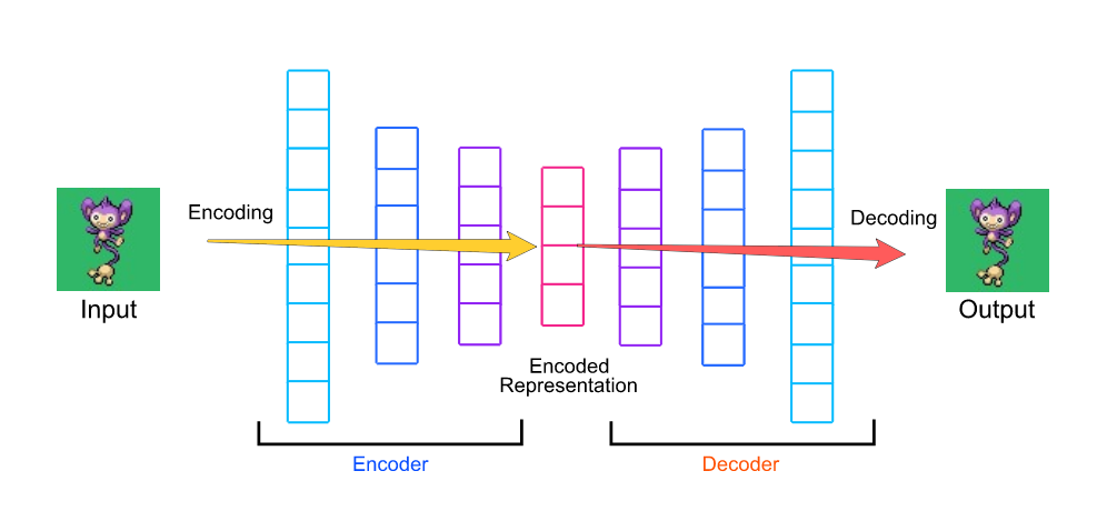
An autoencoder is a network that learns an alternate representations of some data, for example a set of images. It contains two components:
- An encoder that takes an image as input, and outputs a low-dimensional embedding (representation) of the image.
- A decoder that takes the low-dimensional embedding, and reconstructs the image.
Beyond dimension reduction, an autoencoder is a generative model. It can generate new images not in the training set!
An autoencoder is typically shown like below: (image from https://hackernoon.com/how-to-autoencode-your-pok%C3%A9mon-6b0f5c7b7d97 )
Here is an example of a convolutional autoencoder: an autoencoder that uses solely convolutional layers:
class Autoencoder(nn.Module):
    def __init__(self):
        super(Autoencoder, self).__init__()
        self.encoder = nn.Sequential(
            nn.Conv2d(1, 16, 3, stride=2, padding=1),
            nn.ReLU(),
            nn.Conv2d(16, 32, 3, stride=2, padding=1),
            nn.ReLU(),
            nn.Conv2d(32, 64, 7)
        )
        self.decoder = nn.Sequential(
            nn.ConvTranspose2d(64, 32, 7),
            nn.ReLU(),
            nn.ConvTranspose2d(32, 16, 3, stride=2, padding=1, output_padding=1),
            nn.ReLU(),
            nn.ConvTranspose2d(16, 1, 3, stride=2, padding=1, output_padding=1),
            nn.Sigmoid()
        )

    def forward(self, x):
        x = self.encoder(x)
        x = self.decoder(x)
        return x
Notice that the final activation on the decoder is a sigmoid activation. The reason is that we normalize the pixels to be between 0 and 1. A sigmoid gives us results in the same range.
Training an Autoencoder
How do we train an autoencoder? How do we know what kind of "encoder" and "decoder" we want?
For one, if we pass an image through the encoder, then pass the result through the decoder, we should get roughly the same image back. Ideally, reducing the dimensionality and then generating the image should give us the same result!
We use a loss function called MSELoss, which
computes the square error at every pixel.
Beyond using a different loss function, the training
scheme is roughly the same. Note that in the code below,
we are using a new optimizer called Adam.
We switched to this optimizer not because it is specifically used for autoencoders, but because this is the optimizer that people tend to use in practice for convolutional neural networks. Feel free to use Adam for your other convolutional networks.
We are also saving the reconstructed images of the last iteration in every epoch. We want to look at these reconstructions at the end of training.
def train(model, num_epochs=5, batch_size=64, learning_rate=1e-3):
    torch.manual_seed(42)
    criterion = nn.MSELoss()
    optimizer = torch.optim.Adam(model.parameters(), lr=learning_rate, weight_decay=1e-5)
    train_loader = torch.utils.data.DataLoader(mnist_data, batch_size=batch_size, shuffle=True)
    outputs = []
    for epoch in range(num_epochs):
        for data in train_loader:
            img, label = data
            recon = model(img)
            loss = criterion(recon, img)
            loss.backward()
            optimizer.step()
            optimizer.zero_grad()

        print('Epoch:{}, Loss:{:.4f}'.format(epoch+1, float(loss)))
        outputs.append((epoch, img, recon),)
    return outputs
Now, we can train this network.
model = Autoencoder()
max_epochs = 20
outputs = train(model, num_epochs=max_epochs)
The loss goes down as we train, meaning that our reconstructed images look more and more like the actual images!
Let's look at the training progression: that is, the reconstructed images at various points of training:
for k in range(0, max_epochs, 5):
    plt.figure(figsize=(9, 2))
    imgs = outputs[k][1].detach().numpy()
    recon = outputs[k][2].detach().numpy()
    for i, item in enumerate(imgs):
        if i >= 9: break
        plt.subplot(2, 9, i+1)
        plt.imshow(item[0])

    for i, item in enumerate(recon):
        if i >= 9: break
        plt.subplot(2, 9, 9+i+1)
        plt.imshow(item[0])


At first, the reconstructed images look nothing like the originals. Rather, the reconstructions look more like the average of some training images. As training progresses, our reconstructions are clearer.
Structure in the Embeddings
Since we are drastically reducing the dimensionality of the image, there has to be some kind of structure in the embedding space. That is, the network should be able to "save" space by mapping similar images to similar embeddings.
We will demonstrate the structure of the embedding space by hving some fun with our autoencoders. Let's begin with two images in our training set. For now, we'll choose images of the same digit.
imgs = outputs[max_epochs-1][1].detach().numpy()
plt.subplot(1, 2, 1)
plt.imshow(imgs[0][0])
plt.subplot(1, 2, 2)
plt.imshow(imgs[8][0])

We will then compute the low-dimensional embeddings of both images, by applying the encoder:
x1 = outputs[max_epochs-1][1][0,:,:,:] # first image
x2 = outputs[max_epochs-1][1][8,:,:,:] # second image
x = torch.stack([x1,x2])     # stack them together so we only call `encoder` once
embedding = model.encoder(x)
e1 = embedding[0] # embedding of first image
e2 = embedding[1] # embedding of second image
Now we will do something interesting. Not only are we goign to run the
decoder on those two embeddings e1 and e2, we are also going to interpolate
between the two embeddings and decode those as well!
embedding_values = []
for i in range(0, 10):
    e = e1 * (i/10) + e2 * (10-i)/10
    embedding_values.append(e)
embedding_values = torch.stack(embedding_values)

recons = model.decoder(embedding_values)
Let's plot the reconstructions of each interpolated values. The original images are shown below too:
plt.figure(figsize=(10, 2))
for i, recon in enumerate(recons.detach().numpy()):
    plt.subplot(2,10,i+1)
    plt.imshow(recon[0])
plt.subplot(2,10,11)
plt.imshow(imgs[8][0])
plt.subplot(2,10,20)
plt.imshow(imgs[0][0])

Notice that there is a smooth transition between the two images! The middle images are likely new, in that there are no training images that are exactly like any of the generated images.
As promised, we can do the same thing with two images containing different digits. There should be a smooth transition between the two digits.
def interpolate(index1, index2):
    x1 = mnist_data[index1][0]
    x2 = mnist_data[index2][0]
    x = torch.stack([x1,x2])
    embedding = model.encoder(x)
    e1 = embedding[0] # embedding of first image
    e2 = embedding[1] # embedding of second image


    embedding_values = []
    for i in range(0, 10):
        e = e1 * (i/10) + e2 * (10-i)/10
        embedding_values.append(e)
    embedding_values = torch.stack(embedding_values)

    recons = model.decoder(embedding_values)

    plt.figure(figsize=(10, 2))
    for i, recon in enumerate(recons.detach().numpy()):
        plt.subplot(2,10,i+1)
        plt.imshow(recon[0])
    plt.subplot(2,10,11)
    plt.imshow(x2[0])
    plt.subplot(2,10,20)
    plt.imshow(x1[0])

interpolate(0, 1)

interpolate(1, 10)

interpolate(4, 5)

interpolate(20, 30)
