Regularization
In the last few weeks we discussed the idea of overfitting, where a neural network model learns about the quirks of the training data, rather than information that is generalizable to the task at hand. We also briefly discussed idea of underfitting, but not in as much depth.
The reason is that nowadays, practioners tend to avoid underfitting altogether by opting for more powerful models. Since computation is (relatively) cheap, and overfitting is much easier to detect, it is more straightforward to build a high-capacity model and use known techniques to prevent overfitting. If you're not overfitting, you can opt for a more high-capacity model, so detecting overfitting becomes a more important problem than detecting underfitting.
We've already discussed several strategies for detecting overfitting:
- Use a larger training set
- Use a smaller network
- Weight-sharing (as in convolutional neural networks)
- Early stopping
Some of these are more practical than others. For example, collecting a larger training set may be impractical or expensive in practice. Using a smaller network means that we need to restart training, rather than use what we already know about hyperparameters and appropriate weights.
Early stopping was introduced in assignment 2, where we did not use the final trained weights as our ``final'' model. Instead, we used a model (a set of weights) from a previous iteration of training that did not yet overfit.
These are only some of the techniques for preventing overfitting. We'll discuss more techniques today, including:
- Data Augmentation
- Data Normalization
- Model Averaging
- Dropout
We will use the MNIST digit recognition problem as a running example. Since we are studying overfitting, I will artificially reduce the number of training examples to 200.
import torch
import torch.nn as nn
import torch.nn.functional as F
import torch.optim as optim
import matplotlib.pyplot as plt
from torchvision import datasets, transforms

# for reproducibility
torch.manual_seed(1)

mnist_data = datasets.MNIST('data', train=True, download=True, transform=transforms.ToTensor())
mnist_data = list(mnist_data)
mnist_train = mnist_data[:20]     #  20 train images
mnist_val   = mnist_data[100:5100] # 2000 validation images
We will also use the MNISTClassifier from last week as our base model:
class MNISTClassifier(nn.Module):
    def __init__(self):
        super(MNISTClassifier, self).__init__()
        self.layer1 = nn.Linear(28 * 28, 50)
        self.layer2 = nn.Linear(50, 20)
        self.layer3 = nn.Linear(20, 10)
    def forward(self, img):
        flattened = img.view(-1, 28 * 28)
        activation1 = F.relu(self.layer1(flattened))
        activation2 = F.relu(self.layer2(activation1))
        output = self.layer3(activation2)
        return output
And of course, our training code, with minor modifications that we will explain as we go along.
def train(model, train, valid, batch_size=20, num_iters=1, learn_rate=0.01, weight_decay=0):
    train_loader = torch.utils.data.DataLoader(train,
                                               batch_size=batch_size,
                                               shuffle=True) # shuffle after every epoch
    criterion = nn.CrossEntropyLoss()
    optimizer = optim.SGD(model.parameters(), lr=learn_rate, momentum=0.9, weight_decay=weight_decay)

    iters, losses, train_acc, val_acc = [], [], [], []

    # training
    n = 0 # the number of iterations
    while True:
        if n >= num_iters:
            break
        for imgs, labels in iter(train_loader):
            model.train()
            out = model(imgs)             # forward pass
            loss = criterion(out, labels) # compute the total loss
            loss.backward()               # backward pass (compute parameter updates)
            optimizer.step()              # make the updates for each parameter
            optimizer.zero_grad()         # a clean up step for PyTorch

            # save the current training information
            if n % 10 == 9:
                iters.append(n)
                losses.append(float(loss)/batch_size)             # compute *average* loss
                train_acc.append(get_accuracy(model, train)) # compute training accuracy
                val_acc.append(get_accuracy(model, valid))  # compute validation accuracy
            n += 1

    # plotting
    plt.figure(figsize=(10,4))
    plt.subplot(1,2,1)
    plt.title("Training Curve")
    plt.plot(iters, losses, label="Train")
    plt.xlabel("Iterations")
    plt.ylabel("Loss")

    plt.subplot(1,2,2)
    plt.title("Training Curve")
    plt.plot(iters, train_acc, label="Train")
    plt.plot(iters, val_acc, label="Validation")
    plt.xlabel("Iterations")
    plt.ylabel("Training Accuracy")
    plt.legend(loc='best')
    plt.show()

    print("Final Training Accuracy: {}".format(train_acc[-1]))
    print("Final Validation Accuracy: {}".format(val_acc[-1]))


train_acc_loader = torch.utils.data.DataLoader(mnist_train, batch_size=100)
val_acc_loader = torch.utils.data.DataLoader(mnist_val, batch_size=1000)

def get_accuracy(model, data):
    correct = 0
    total = 0
    model.eval()
    for imgs, labels in torch.utils.data.DataLoader(data, batch_size=64):
        output = model(imgs) # We don't need to run F.softmax
        pred = output.max(1, keepdim=True)[1] # get the index of the max log-probability
        correct += pred.eq(labels.view_as(pred)).sum().item()
        total += imgs.shape[0]
    return correct / total
Without any intervention, our model gets to about 52-53% accuracy on the validation set.
model = MNISTClassifier()
train(model, mnist_train, mnist_val, num_iters=500)

Data Augmentation
While it is often expensive to gather more data, we can make alterations to our existing dataset, and treat the altered data set as a new training data point. Common ways of obtaining new (image) data include:
- Flipping each image horizontally or vertically (won't work for digit recognition, but might for other tasks)
- Shifting each pixel a little to the left or right
- Rotating the images a little
- Adding noise to the image
... or even a combination of the above. For demonstration purposes, let's randomly rotate our digits a little to get new training samples.
Here are the 20 images in our training set:
def show20(data):
    plt.figure(figsize=(10,2))
    for n, (img, label) in enumerate(data):
        if n >= 20:
            break
        plt.subplot(2, 10, n+1)
        plt.imshow(img)

mnist_imgs = datasets.MNIST('data', train=True, download=True)
show20(mnist_imgs)

Here are the 20 images in our training set, each rotated randomly, by up to 25 degrees.
mnist_new = datasets.MNIST('data', train=True, download=True, transform=transforms.RandomRotation(25))
show20(mnist_new)

If we apply the transformation again, we can get images with different rotations:
mnist_new = datasets.MNIST('data', train=True, download=True, transform=transforms.RandomRotation(25))
show20(mnist_new)

We can augment our data set by, say, randomly rotating each training data point 100 times:
augmented_train_data = []

my_transform = transforms.Compose([
    transforms.RandomRotation(25),
    transforms.ToTensor(),
])

for i in range(100):
    mnist_new = datasets.MNIST('data', train=True, download=True, transform=my_transform)
    for j, item in enumerate(mnist_new):
        if j >= 20:
            break
        augmented_train_data.append(item)

len(augmented_train_data)
We obtain a better validation accuracy after training on our expanded dataset.
model = MNISTClassifier()
train(model, augmented_train_data, mnist_val, num_iters=500)

Data Normalization
Another common practice is to normalize the data so that the mean and standard deviation is constant across each channel. For example, in your assignment 2 code, we used the following transform:
transforms.Normalize((0.5, 0.5, 0.5), (0.5, 0.5, 0.5))
This transform standardizes each pixel intensity to have mean 0.5 and standard deviation 0.5.
Weight Decay
A more interesting technique that prevents overfitting is the idea of weight decay. The idea is to penalize large weights. We avoid large weights, because large weights mean that the prediction relies a lot on the content of one pixel, or on one unit. Intuitively, it does not make sense that the classification of an image should depend heavily on the content of one pixel, or even a few pixels.
Mathematically, we penalize large weights by adding an extra term to the loss function, the term can look like the following:
- $L^1$ regularization: $\sum_k |w_k|$
- Mathematically, this term encourages weights to be exactly 0
- $L^2$ regularization: $\sum_k w_k^2$
- Mathematically, in each iteration the weight is pushed towards 0
- Combination of $L^1$ and $L^2$ regularization: add a term $\sum_k |w_k| + w_k^2$ to the loss function.
In PyTorch, weight decay can also be done automatically inside an optimizer. The parameter weight_decay
of optim.SGD and most other optimizers uses $L^2$ regularization for weight decay. The value of the
weight_decay parameter is another tunable hyperparameter.
model = MNISTClassifier()
train(model, mnist_train, mnist_val, num_iters=500, weight_decay=0.001)

Dropout
Yet another way to prevent overfitting is to build many models, then average their predictions at test time. Each model might have a different set of initial weights.
We won't show an example of model averaging here. Instead, we will show another idea that sounds drastically different on the surface.
This idea is called dropout: we will randomly "drop out", "zero out", or "remove" a portion of neurons from each training iteration.
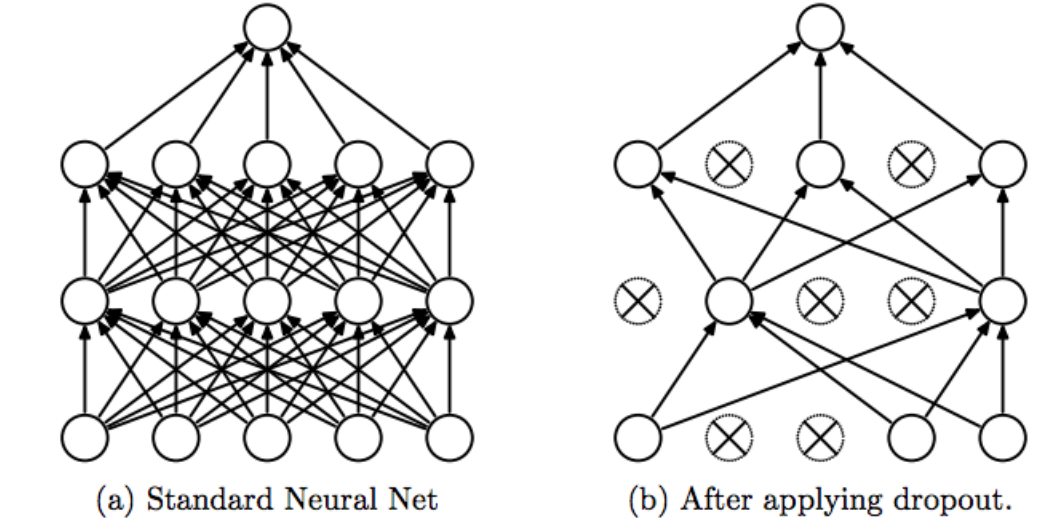
In different iterations of training, we will drop out a different set of neurons.
The technique has an effect of preventing weights from being overly dependent on each other: for example for one weight to be unnecessarily large to compensate for another unnecessarily large weight with the opposite sign. Weights are encouraged to be "more independent" of one another.
During test time though, we will not drop out any neurons; instead we will use
the entire set of weights. This means that our training time and test time behaviour
of dropout layers are different. In the code for the function train and get_accuracy,
we use model.train() and model.eval() to flag whether we want the model's training behaviour,
or test time behaviour.
While unintuitive, using all connections is a form of model averaging! We are effectively averaging over many different networks of various connectivity structures.
class MNISTClassifierWithDropout(nn.Module):
    def __init__(self):
        super(MNISTClassifierWithDropout, self).__init__()
        self.layer1 = nn.Linear(28 * 28, 50)
        self.layer2 = nn.Linear(50, 20)
        self.layer3 = nn.Linear(20, 10)
        self.dropout1 = nn.Dropout(0.2) # drop out layer with 20% dropped out neuron
        self.dropout2 = nn.Dropout(0.2)
        self.dropout3 = nn.Dropout(0.2)
    def forward(self, img):
        flattened = img.view(-1, 28 * 28)
        activation1 = F.relu(self.layer1(self.dropout1(flattened)))
        activation2 = F.relu(self.layer2(self.dropout2(activation1)))
        output = self.layer3(self.dropout3(activation2))
        return output

model = MNISTClassifierWithDropout()
train(model, mnist_train, mnist_val, num_iters=500)
