Convolutional Neural Networks
So far, we have used feed-forward neural networks with fully connected layers. While fully connected layers are useful, they are not always what we want.
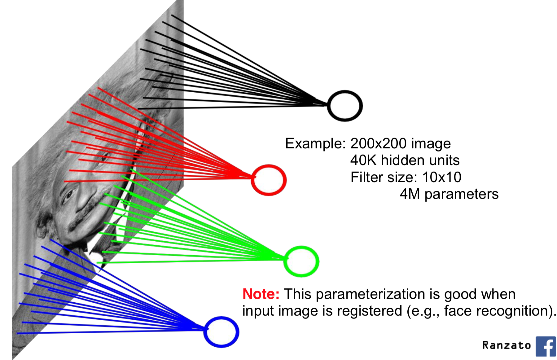
Specifically, fully connected layers require a lot of connections. Suppose we are trying to determine whether an image of size $200 \times 200$ contains a cat. Our input layer would need to have $200 \times 200 = 40000$ units, one for each pixel. A fully connected layer between the input and the first hidden layer with, say, 500 hidden units will require a whopping $40000 \times 500 =$ 20 million connections!
The large number of connections means several things. For one, computing predictions will require a lot of processing time. For another, we will have a large number of weights, making our network very high capacity. The high capacity of the network means that we will need a large number of training examples to avoid overfitting.
There is also one other issue. What happens if our image is shifted a little, say one pixel to the left? Even though the change is minor from our point of view, the intensity at each pixel location could change drastically. We can get a completely different prediction from our network.
Since there are many well-written resources on convolutional neural networks, these notes will be terser than usual.
Locally Connected Layers
What we will do is look for local features. For example, features like edges, textures, and other patterns depend only on pixel intensities in a small region. Here is an example of a locally connected layer:
Each unit in the (first) hidden layer detects patterns in a small portion of the input image. This way, we have fewer connections (and therefore weights) between the input and the first hidden layer.
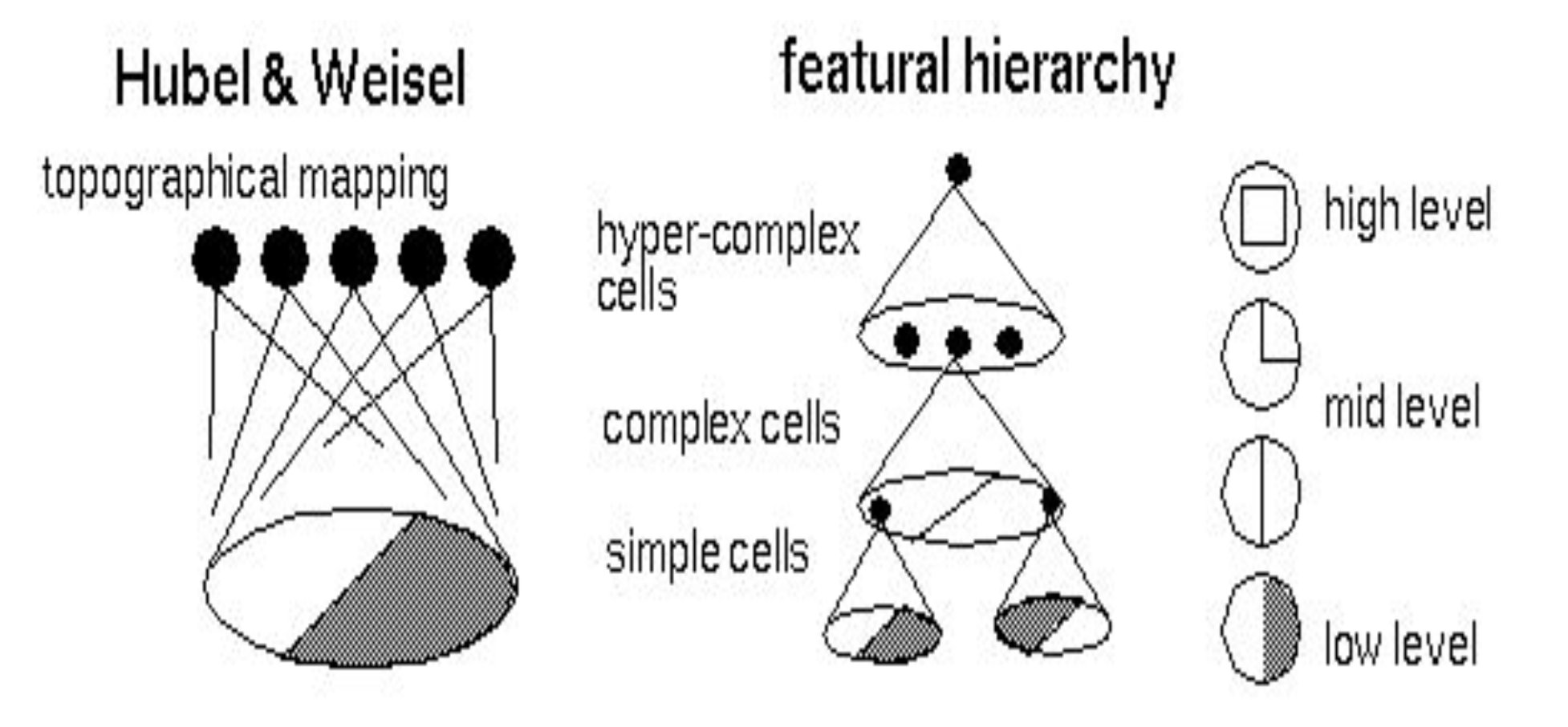
There is biological evidence that the (biological) neural connectivity in the visual cortex works the same way, where neurons detect features that occur in a small region of our receptive field. Neurons close to the retina detect simple patterns like edges. Neurons that receive information from these simple cells detect more complicated patterns. Neurons in even higher layers detect even more complicated patterns.
Weight Sharing
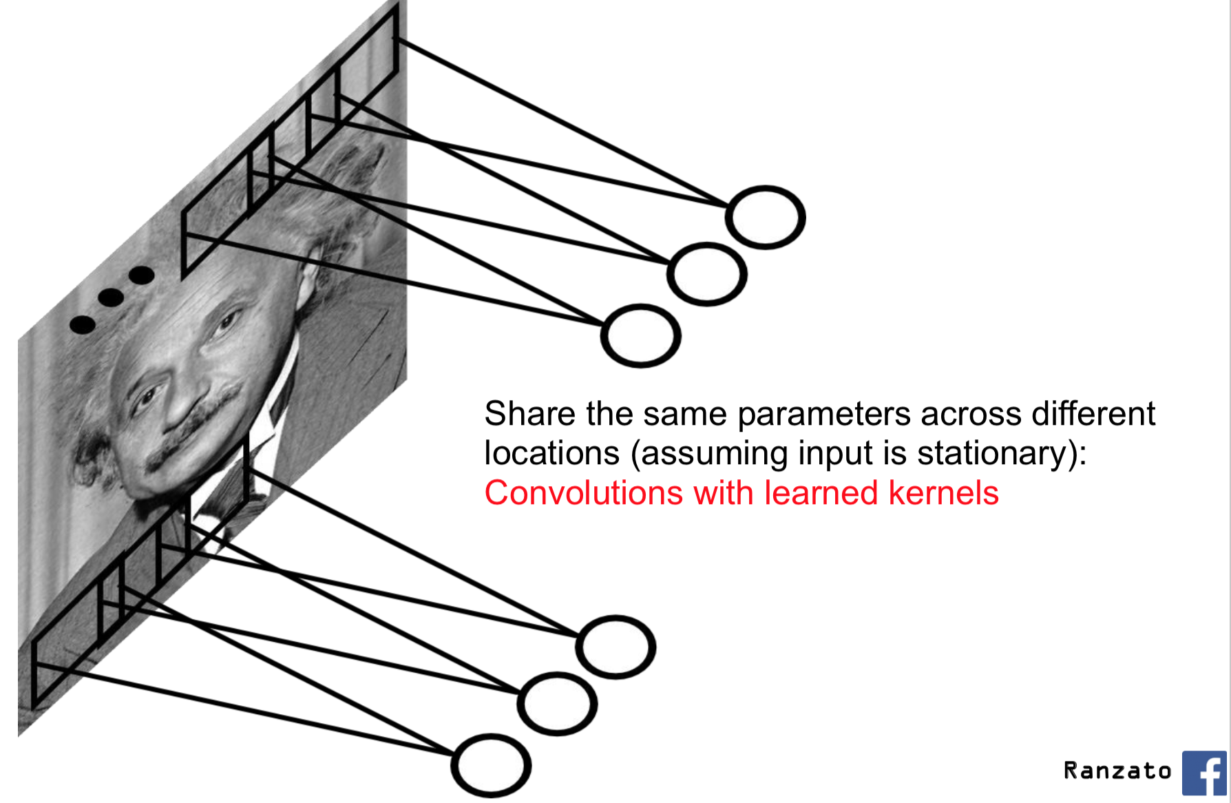
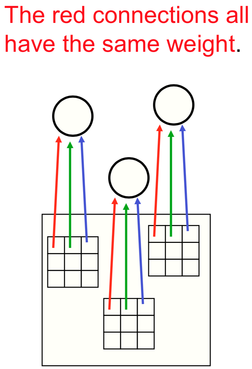
If we know how to detect a local feature in one region of the image -- say, an edge in a certain orientation -- then we know how to detect that feature in other regions of the image. This is the idea behind weight sharing: we will share the same parameters across different locations in an image.
Filters in Computer Vision
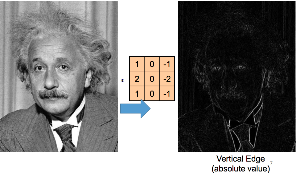
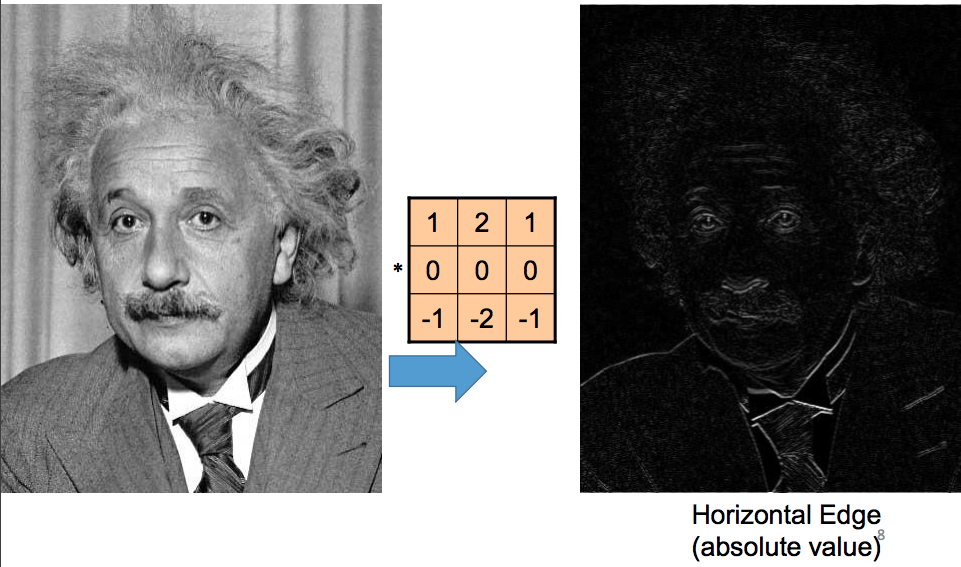
People have used the idea of convolutional filters in computer vision even before the rise of machine learning. They hand-coded filters that can detect simple features, for example edges in various orientations:
The Convolutional Layer
Recall that in PyTorch, we can create a fully-connected layer between successive layers like this:
import torch.nn as nn

# fully-connected layer between a lower layer of size 100, and
# a higher layer of size 30
fc = nn.Linear(100, 30)
We've applied a layer like this as follows:
import torch
x = torch.randn(100) # create a tensor of shape [100]
y = fc(x)            # apply the fully conected layer `fc` to x
y.shape
In PyTorch, we can create a convolutional layer using nn.Conv2d:
conv = nn.Conv2d(in_channels=3,  # number of channels in the input (lower layer)
                 out_channels=7, # number of channels in the output (next layer)
                 kernel_size=5)  # size of the kernel or receiptive field
The conv layer expects as input a tensor in the format "NCHW", meaning that
the dimensions of the tensor should follow the order:
- batch size
- channel
- height
- width
For example, we can emulate a batch of 32 colour images, each of size 128x128, like this:
x = torch.randn(32, 3, 128, 128)
y = conv(x)
y.shape
The output tensor is also in the "NCHW" format. We still have 32 images, and 7 channels
(consistent with out_channels of conv), and of size 124x124. If we added the appropriate
padding to conv, namely padding = kernel_size // 2, then our output width and height should
be consistent with the input width and height:
conv2 = nn.Conv2d(in_channels=3,
                  out_channels=7,
                  kernel_size=5,
                  padding=2)

x = torch.randn(32, 3, 128, 128)
y = conv2(x)
y.shape
To further illustrate the formatting, let's apply the (random, untrained) convolution conv2 to
a real image. First, we load the image:
import matplotlib.pyplot as plt
import numpy as np

img = plt.imread("imgs/dog_mochi.png")[:, :, :3]
plt.imshow(img)
Then, we convert the image into a PyTorch tensor of the appropriate shape.
x = torch.from_numpy(img) # turn img into a PyTorch tensor
print(x.shape)
x = x.permute(2,0,1)      # move the channel dimension to the beginning
print(x.shape)
x = x.reshape([1, 3, 350, 210]) # add a dimension for batching
print(x.shape)
Even when our batch size is 1, we still need the first dimension so that the input follows the "NCHW" format.
y = conv2(x)           # apply the convolution
y = y.detach().numpy() # convert the result into numpy
y = y[0]               # remove the dimension for batching

# normalize the result to [0, 1] for plotting
y_max = np.max(y)
y_min = np.min(y)
img_after_conv = y - y_min / (y_max - y_min)
img_after_conv.shape
Let's plot the 7 channels one by one:
plt.figure(figsize=(14,4))
for i in range(7):
    plt.subplot(1, 7, i+1)
    plt.imshow(img_after_conv[i])

If we were to run a neural network, these would be the unit outputs (prior to applying the activation function).
Pooling Layers
pool = nn.MaxPool2d(2, 2)
y = conv2(x)
z = pool(y)
z.shape
Convolutional Networks in PyTorch
In assignment 2, we created the following network. We can understand this network now!
class LargeNet(nn.Module):
    def __init__(self):
        super(LargeNet, self).__init__()
        self.name = "large"
        self.conv1 = nn.Conv2d(3, 5, 5)
        self.pool = nn.MaxPool2d(2, 2)
        self.conv2 = nn.Conv2d(5, 10, 5)
        self.fc1 = nn.Linear(10 * 5 * 5, 32)
        self.fc2 = nn.Linear(32, 1)

    def forward(self, x):
        x = self.pool(F.relu(self.conv1(x)))
        x = self.pool(F.relu(self.conv2(x)))
        x = x.view(-1, 10 * 5 * 5)
        x = F.relu(self.fc1(x))
        x = self.fc2(x)
        x = x.squeeze(1) # Flatten to [batch_size]
        return x
This network has two convolutional layers: conv1 and conv2.
- The first convolutional layer
conv1requires an input with 3 channels, outputs 5 channels, and has a kernel size of5x5. We are not adding any zero-padding. - The second convolutional layer
conv1requires an input with 5 channels, outputs 10 channels, and has a kernel size of (again)5x5. We are not adding any zero-padding.
In the forward function we see that the convolution operations are always
followed by the usual ReLU activation function, and a pooling operation.
The pooling operation used is max pooling, so each pooling operation
reduces the width and height of the neurons in the layer by half.
Because we are not adding any zero padding, we end up with 10 * 5 * 5 hidden units
after the second convolutional layer. These units are then passed to two fully-connected
layers, with the usual ReLU activation in between.
Notice that the number of channels grew in later convolutional layers! However, the number of hidden units in each layer is still reduced because of the pooling operation:
- Initial Image Size: $3 \times 32 \times 32 = 3072$
- After
conv1: $5 \times 28 \times 28$ - After Pooling: $5 \times 14 \times 14 = 980$
- After
conv2: $10 \times 10 \times 10$ - After Pooling: $10 \times 5 \times 5 = 250$
- After
fc1: $32$ - After
fc2: $1$
This pattern of doubling the number of channels with every pooling / strided convolution is common in convolutional architectures. It is used to avoid loss of too much information within a single convolution.
AlexNet in PyTorch
Convolutional networks are very commonly used, meaning that there are often alternatives to training convolutional networks from scratch. In particular, researchers often release both the architecture and the weights of the networks they train.
As an example, let's look at the AlexNet model, whose trained weights are included in torchvision.
AlexNet was trained to classify images into one of many categories.
The AlexNet can be imported like below.
import torchvision.models

alexNet = torchvision.models.alexnet(pretrained=True)
alexNet
Notice that the AlexNet model is split into two parts. There is a component that computes "features" using convolutions.
alexNet.features
There is also a component that classifies the image based on the computed features.
alexNet.classifier
AlexNet Features
The first network can be used independently of the second. Specifically, it can be used to compute a set of features that can be used later on. This idea of using neural network activation features to represent images is an extremely important one, so it is important to understand the idea now.
If we take our image x from earlier and apply it to the alexNet.features network,
we get some numbers like this:
features = alexNet.features(x)
features.shape
The set of numbers in features is another way of representing our image x. Recall that
our initial image x was also represented as a tensor, also a set of numbers representing
pixel intensity. Geometrically speaking, we are using points in a high-dimensional space to
represent the images. In our pixel representation, the axes in this high-dimensional space
were different pixels. In our features representation, the axes are not as easily
interpretable.
But we will want to work with the features representation, because this representation
makes classification easier. This representation organizes images in a more "useful" and
"semantic" way than pixels.
Let me be more specific:
this set of features was trained on image classification. It turns out that
these features can be useful for performing other image-related tasks as well!
That is, if we want to perform an image classification task of our own (for example,
classifying cancer biopsies, which is nothing like what AlexNet was trained to do),
we might compute these AlexNet features, and then train a small model on top of those
features. We replace the classifier portion of AlexNet, but keep its features
portion intact.
Somehow, through being trained on one type of image classification problem, AlexNet learned something general about representing images.
AlexNet First Convolutions
Since we have a trained model, we might as well visualize outputs of a trained convolution, to contrast with the untrained convolution we visualized earlier.
Here is the first convolution of AlexNet, applied to our image of Mochi.
alexNetConv = alexNet.features[0]
y = alexNetConv(x)
The output is a $1 \times 64 \times 86 \times 51$ tensor.
y = y.detach().numpy()
y = (y - y.min()) / (y.max() - y.min())
y.shape
We can visualize each channel independently.
plt.figure(figsize=(10,10))
for i in range(64):
    plt.subplot(8, 8, i+1)
    plt.imshow(y[0, i])
