Neural Network Terminology
Last week, we introduced a lot of neural network terminology. Let's review some of these terms, and add some more useful terms to our vocabulary.
Most of the figures here are from http://cs231n.github.io/neural-networks-1/
The Artificial Neurons
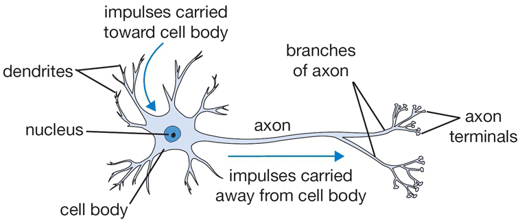
Neurons pass information from one to another using action potentials. They connect with one another at synapes, which are junctions between one neuron's axon and another's dendrite. Information flows from:
- the dendrite
- to the cell body
- through the axons
- to a synapse connecting the axon to the dendrite of the next neuron.
The biological neuron is very complicated, and has many biochemical elements that are difficult to simulate. Instead, we use a simplified model of the neuron that only models the information flow.
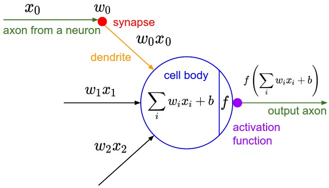
A neuron receives the activation values $x_i$ from neurons connected to its dendrites. The neuron needs to combine those activations. However, the connections between neurons can be weak or strong. The strength is represented by $w_i$, and the amount of information "received" by the neuron is the product $w_i x_i$. The total contributions are combined together, along with a bias $b$, forming the sum $b + \sum_i w_i x_i$. This value is then passed to a non-linear activation function $f$ to produce the output $f(b+\sum_i w_i x_i)$. This is the activation of our neuron, and is the value passed to other neurons connected to its axon.
The Activation Function
We glossed over the idea of the activation function last time. The biological neuron's output is certainly not a linear combination of its inputs, so a nonlinear activation function is well motivated. More importantly, if we do not have any kind of non-linearity, then we will only be able to learn linear relationships between input and output: a composition of linear functions is still a linear function. Nonlinear activation functions are a requirement if we want to perform interesting nonlinear tasks.
So, what non-linear activation functions do we choose?
Recall our code from last time:
import torch
import torch.nn as nn
import torch.nn.functional as F
from torchvision import datasets, transforms
import matplotlib.pyplot as plt # for plotting

torch.manual_seed(1) # set the random seed

class Pigeon(nn.Module):
    def __init__(self):
        super(Pigeon, self).__init__()
        self.layer1 = nn.Linear(28 * 28, 30)
        self.layer2 = nn.Linear(30, 1)
    def forward(self, img):
        flattened = img.view(-1, 28 * 28)
        activation1 = self.layer1(flattened)
        activation1 = F.relu(activation1)
        activation2 = self.layer2(activation1)
        return activation2

pigeon = Pigeon()

# load the data
mnist_train = datasets.MNIST('data', train=True, download=True)
mnist_train = list(mnist_train)[:2000]
img_to_tensor = transforms.ToTensor()

# make predictions for the first 10 images in mnist_train
for k, (image, label) in enumerate(mnist_train[:10]):
    print(torch.sigmoid(pigeon(img_to_tensor(image))))
The model pigeon is actually a two-layer neural network.
Activations in each layer is stored together:
for example activation1 in the Pigeon.forward method is a
PyTorch tensor of dimension 30.
We used two different activation functions for the two layers:
We used the rectifier function (F.relu) for the outputs of
the first layer, and the sigmoid function (torch.sigmoid)
for the output (yes, singular) of the second layer.
Rectifier function
A rectifier (or a linear rectifier) looks like this:
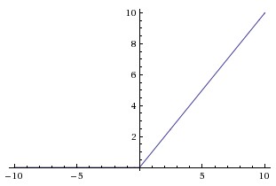
The function is linear when the activation is above zero, and is equal to zero otherwise. An artificial neuron unit that uses the rectifier function as its non-linearity is called a rectified linear unit (ReLU).
Most machine learning practitioners nowadays (early 2019) use ReLU units for intermediate layers of a neural network. The mathematics of the ReLU unit is extremely simple, so networks with ReLU units are easier to optimize than those using sigmoid activation.
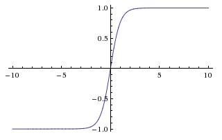
Sigmoid function
A sigmoid function, denoted $\sigma$, looks like this:
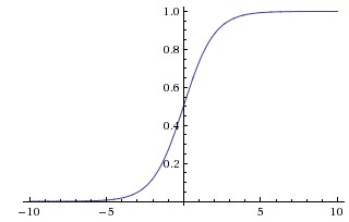
The sigmoid function has a tilted "S" shape, and its output is always between 0 and 1. In fact, outputs of sigmoid functions are interpretable as probabilities! Practitioners often use sigmoid functions to turn a real number output into a probability. This is exactly what we have done above:
out = pigeon(img_to_tensor(image)) # `out` is an arbitrary floating-point number
prob = torch.sigmoid(out)          # `prob` is between 0 and 1
print("Output:", out, "Probability:", prob)
Tanh function
We haven't used the tanh activation function yet in this course. The tanh function is a variation of the sigmoid function. The output of the tanh function is always between -1 and 1 (instead of 0 and 1)
We probably won't use the tanh activation function in this course, but it is an alternative to the ReLU activation.
Parameters
The parameters of a network are the numbers that can be tuned
to train the network. The parameters include the weights
and biases.
We can count the number of parameters in our model pigeon:
- In the first layer, there are
28*28input neurons, and30hidden neurons. This means that there are28*28*30weights (one for each input-hidden neuron pair), and30biases. - In the second layer, there are
30hidden neurons, and1output neuron. This means that there are30*1weights, and1bias.
So the total number of parameters of the model pigeon is
(28 * 28 * 30) + 30 + (30 * 1) + 30
We often use the term weights synonymously with the term parameters,
to denote both weights and biases of a neural network.
This is because biases can be thought of as a weight from a neuron that always
outputs an activation of 1. So by introducing a variable $x_0 = 1$, we can rewrite
$f(b + \sum_{i=1}^{M} w_i x_i)$ as $f(\sum_{i=0}^{M} w_i x_i)$.
A larger neural network typically has higher capacity, meaning that it is capable of solving more complex problems. However, larger capacity neural networks take more resources to train. Not only do we need the memory to store the additional weights, we also need more time and processing power to compute updates for those weights during training.
Neural Network Architecture
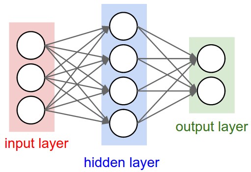
An architecture describes the neurons and their connectivity in the network. The connectivity of biological neurons is highly complex, with each neuron connected to tens of thousands of other neurons! Artificial neural networks are not as well-connected. Moreover, the connections patterns of artificial neurons tend to be simpler. Thus far, we have introduced a feed-forward, fully-connected network, also known as a multi-layer perceptron.
Normally, when we count the number of layers in a neural network, we do not count the input layer. This way, the number of layers equal to the number of sets of weights and biases.
For example, this is a two-layer neural network:
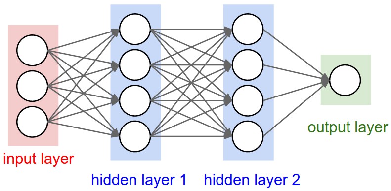
And this is a three-layer neural network:
Training
Recall that we train a neural network to adjust its parameters.
A loss function $L(actual, predicted)$ computes how "bad" a predictions was, compared to the ground truth value for the input. A large loss means that the network's prediction differs from the ground truth, whereas a small loss means that the network's prediction is similar to the ground truth.
As mentioned last time, the loss function transforms a problem of finding good weights to perform a task, into an optimization problem: finding the weights that minimize the loss function (or the average value of the loss function across some training data). In each iteration, we are taking one step towards solving the optimization problem:
$min_{weights} L(prediction, actual, weights)$
The transformation of learning problems into optimization problems will be a recurring theme as you study more machine learning models.
An optimizer determines, based on the loss function, how -- and how much -- each parameter should change. The optimizer solves the credit assignment problem: how do we assign credit (blame) to the parameters when the network performs poorly?
The solution to the credit assignment problem is gradient descent, which we will not talk about in this course. You should know that gradient descent uses the gradient of the loss function to compute changes to each parameter. This places restrictions on the kind of loss functions and activation functions we can use. We need to be able to take gradients of the loss function and the activation function with respect to the parameters.
We'll have a more thorough discussion about neural network training next time.
Datasets
A set of labelled data is data whose desired predictions are known. Recall that last time, we used a portion of our labelled data for training, and a different portion of our data for testing. In general, these two portions of data are called the training set and the test set.
We use the training set to train the network: to compare our network's predictions against the ground truth, and make adjustments to the weights of the network.
We use the test set to get a more accurate assessment of how well our network might do on new data that it has never seen before. If a network performs well on the training set, but poorly on the test set, then the network has overfit to the training set.
For standard data sets like MNIST, there are standard train/test splits
that researchers and practitioners share. Although we have been using images
1000 images from mnist_train as our "test set", there is a standard MNIST
test set that we can access like this:
mnist_test = datasets.MNIST('data', train=False, download=True)
The reasons people try to use the same train/test split is because different splits can sometimes have some impact on network performance. (Some test sets might be "easier" than others").