Recurrent Neural Networks
Last time, before the midterm, we discussed using recurrent neural networks to make predictions about sequences. In particular, we treated tweets as a sequence of words. Since tweets can have a variable number of words, we needed an architecture that can take variable-sized sequences as input.
This time, we will use recurrent neural networks to generate sequences. Generating sequences is more involved comparing to making predictions about sequences. However, it is a very interesting task, and many students chose sequence-generation tasks for their projects.
Much of today's content is an adaptation of the "Practical PyTorch" github repository [1].
[1] https://github.com/spro/practical-pytorch/blob/master/char-rnn-generation/char-rnn-generation.ipynb
import torch
import torch.nn as nn
import torch.nn.functional as F
import torch.optim as optim
Review
The recurrent neural network architecture from last time looked something like this:
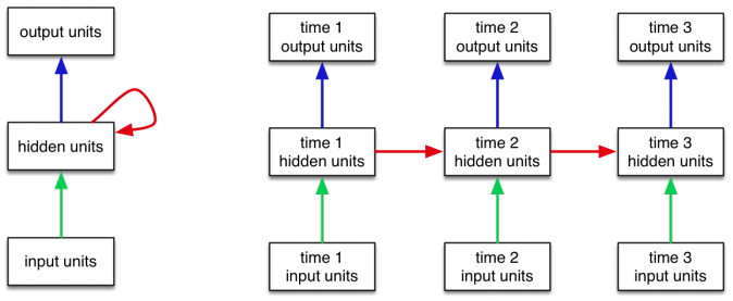
The input sequence is broken down into tokens. We could choose whether to tokenize based on words, or based on characters. The representation of each token (GloVe or one-hot) is processed by the RNN one step at a time to update the hidden (or context) state.
In a predictive RNN, the value of the hidden states is a representation of all the text that was processed thus far. Similarly, in a generative RNN, The value of the hidden state will be a representation of all the text that still needs to be generated. We will use this hidden state to produce the sequence, one token at a time.
Similar to last class we will break up the problem of generating text to generating one token at a time.
We will do so with the help of two functions:
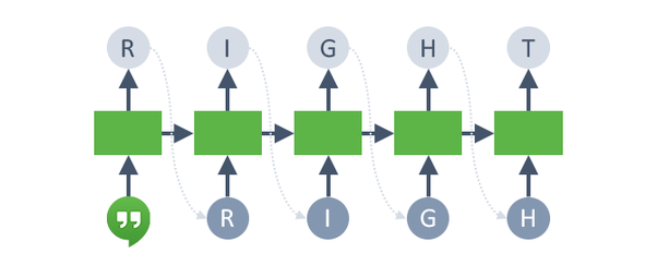
- We need to be able to generate the next token, given the current hidden state. In practice, we get a probability distribution over the next token, and sample from that probability distribution.
- We need to be able to update the hidden state somehow. To do so, we need two piece of information: the old hidden state, and the actual token that was generated in the previous step. The actual token generated will inform the subsequent tokens.
We will repeat both functions until a special "END OF SEQUENCE" token is generated. Here is a pictorial representation of what we will do:
Note that there are several tricky things that we will have to figure out. For example, how do we actually sample the actual token from the probability distribution over tokens? What would we do during training, and how might that be different from during testing/evaluation? We will answer those questions as we implement the RNN.
For now, let's start with our training data.
Data: Donald Trump's Tweets from 2018
The training set we use is a collection of Donald Trump's tweets from 2018. We will only use tweets that are 140 characters or shorter, and tweets that contains more than just a URL. Since tweets often contain creative spelling and numbers, and upper vs lower case characters are read very differently, we will use a character-level RNN.
import csv
tweets = list(line[0] for line in csv.reader(open('trump.csv')))
len(tweets)
There are over 20000 tweets in this collection. Let's look at a few of them, just to get a sense of the kind of text we're dealing with:
print(tweets[100])
print(tweets[1000])
print(tweets[10000])
Generating One Tweet
Normally, when we build a new machine learn model, we want to make sure
that our model can overfit. To that end, we will first build a neural network
that can generate one tweet really well. We can choose any tweet (or any other text)
we want. Let's choose to build an RNN that generates tweet[100].
tweet = tweets[100]
tweet
First, we will need to encode this tweet using a one-hot encoding.
We'll build dictionary mappings
from the character to the index of that character (a unique integer identifier),
and from the index to the character. We'll use the same naming scheme that torchtext
uses (stoi and itos).
For simplicity, we'll work with a limited vocabulary containing
just the characters in tweet[100], plus two special tokens:
<EOS>represents "End of String", which we'll append to the end of our tweet. Since tweets are variable-length, this is a way for the RNN to signal that the entire sequence has been generated.<BOS>represents "Beginning of String", which we'll prepend to the beginning of our tweet. This is the first token that we will feed into the RNN.
The way we use these special tokens will become more clear as we build the model.
vocab = list(set(tweet)) + ["<BOS>", "<EOS>"]
vocab_stoi = {s: i for i, s in enumerate(vocab)}
vocab_itos = {i: s for i, s in enumerate(vocab)}
vocab_size = len(vocab)
Now that we have our vocabulary, we can build the PyTorch model for this problem. The actual model is not as complex as you might think. We actually already learned about all the components that we need. (Using and training the model is the hard part)
class TextGenerator(nn.Module):
    def __init__(self, vocab_size, hidden_size, n_layers=1):
        super(TextGenerator, self).__init__()

        # identiy matrix for generating one-hot vectors
        self.ident = torch.eye(vocab_size)

        # recurrent neural network
        self.rnn = nn.GRU(vocab_size, hidden_size, n_layers, batch_first=True)

        # a fully-connect layer that outputs a distribution over
        # the next token, given the RNN output
        self.decoder = nn.Linear(hidden_size, vocab_size)

    def forward(self, inp, hidden=None):
        inp = self.ident[inp]                  # generate one-hot vectors of input
        output, hidden = self.rnn(inp, hidden) # get the next output and hidden state
        output = self.decoder(output)          # predict distribution over next tokens
        return output, hidden

model = TextGenerator(vocab_size, 64)
Training with Teacher Forcing
At a very high level, we want our RNN model to have a high probability of generating the tweet. An RNN model generates text one character at a time based on the hidden state value. At each time step, we will check whether the mdoel generated the correct character. That is, at each time step, we are trying to select the correct next character out of all the characters in our vocabulary. Recall that this problem is a multi-class classification problem, and we can use Cross-Entropy loss to train our network to become better at this type of problem.
criterion = nn.CrossEntropyLoss()
However, we don't just have a single multi-class classification problem. Instead, we have one classification problem per time-step (per token)! So, how do we predict the first token in the sequence? How do we predict the second token in the sequence?
To help you understand what happens durign RNN training, we'll start with a inefficient training code that shows you what happens step-by-step. We'll start with computing the loss for the first token generated, then the second token, and so on. Later on, we'll switch to a simpler and more performant version of the code.
So, let's start with the first classification problem: the problem of generating
the first token (tweet[0]).
To generate the first token, we'll feed the RNN network (with an initial, empty
hidden state) the "
bos_input = torch.Tensor([vocab_stoi["<BOS>"]]).long().unsqueeze(0)
output, hidden = model(bos_input, hidden=None)
output # distribution over the first token
We can compute the loss using criterion. Since the model is untrained,
the loss is expected to be high. (For now, we won't do anything
with this loss, and omit the backward pass.)
target = torch.Tensor([vocab_stoi[tweet[0]]]).long().unsqueeze(0)
criterion(output.reshape(-1, vocab_size), # reshape to 2D tensor
          target.reshape(-1))             # reshape to 1D tensor
Now, we need to update the hidden state and generate a prediction for the next token. To do so, we need to provide the current token to the RNN. We already said that during test time, we'll need to sample from the predicted probabilty over tokens that the neural network just generated.
Right now, we can do something better: we can use the ground-truth, actual target token. This technique is called teacher-forcing, and generally speeds up training. The reason is that right now, since our model does not perform well, the predicted probability distribution is pretty far from the ground truth. So, it is very, very difficult for the neural network to get back on track given bad input data.
# Use teacher-forcing: we pass in the ground truth `target`,
# rather than using the NN predicted distribution
output, hidden = model(target, hidden)
output # distribution over the second token
Similar to the first step, we can compute the loss, quantifying the difference between the predicted distribution and the actual next token. This loss can be used to adjust the weights of the neural network (which we are not doing yet).
target = torch.Tensor([vocab_stoi[tweet[1]]]).long().unsqueeze(0)
criterion(output.reshape(-1, vocab_size), # reshape to 2D tensor
          target.reshape(-1))             # reshape to 1D tensor
We can continue this process of:
- feeding the previous ground-truth token to the RNN,
- obtaining the prediction distribution over the next token, and
- computing the loss,
for as many steps as there are tokens in the ground-truth tweet.
for i in range(2, len(tweet)):
    output, hidden = model(target, hidden)
    target = torch.Tensor([vocab_stoi[tweet[1]]]).long().unsqueeze(0)
    loss = criterion(output.reshape(-1, vocab_size), # reshape to 2D tensor
                     target.reshape(-1))             # reshape to 1D tensor
    print(i, output, loss)
Finally, with our final token, we should expect to output the "
output, hidden = model(target, hidden)
target = torch.Tensor([vocab_stoi["<EOS>"]]).long().unsqueeze(0)
loss = criterion(output.reshape(-1, vocab_size), # reshape to 2D tensor
                 target.reshape(-1))             # reshape to 1D tensor
print(i, output, loss)
In practice, we don't really need a loop. Recall that in a predictive RNN,
the nn.RNN module can take an entire sequence as input. We can do the
same thing here:
tweet_ch = ["<BOS>"] + list(tweet) + ["<EOS>"]
tweet_indices = [vocab_stoi[ch] for ch in tweet_ch]
tweet_tensor = torch.Tensor(tweet_indices).long().unsqueeze(0)

print(tweet_tensor.shape)

output, hidden = model(tweet_tensor[:,:-1]) # <EOS> is never an input token
target = tweet_tensor[:,1:]                 # <BOS> is never a target token
loss = criterion(output.reshape(-1, vocab_size), # reshape to 2D tensor
                 target.reshape(-1))             # reshape to 1D tensor
Here, the input to our neural network model is the entire
sequence of input tokens (everything from "target.
Our training loop (for learning to generate the single tweet) will therefore
look something like this:
optimizer = torch.optim.Adam(model.parameters(), lr=0.001)
criterion = nn.CrossEntropyLoss()
for it in range(500):
    optimizer.zero_grad()
    output, _ = model(tweet_tensor[:,:-1])
    loss = criterion(output.reshape(-1, vocab_size),
                 target.reshape(-1))
    loss.backward()
    optimizer.step()

    if (it+1) % 100 == 0:
        print("[Iter %d] Loss %f" % (it+1, float(loss)))
The training loss is decreasing with training, which is what we expect.
Generating a Token
At this point, we want to see whether our model is actually learning something. So, we need to talk about how to actually use the RNN model to generate text. If we can generate text, we can make a qualitative asssessment of how well our RNN is performing.
The main difference between training and test-time (generation time) is that we don't have the ground-truth tokens to feed as inputs to the RNN. Instead, we need to actually sample a token based on the neural network's prediction distribution.
But how can we sample a token from a distribution?
On one extreme, we can always take the token with the largest probability (argmax). This has been our go-to technique in other classification tasks. However, this idea will fail here. The reason is that in practice, we want to be able to generate a variety of different sequences from the same model. An RNN that can only generate a single new Trump Tweet is fairly useless.
In short, we want some randomness. We can do so by using the logit outputs from our model to construct a multinomial distribution over the tokens, then and sample a random token from that multinomial distribution.
One natural multinomial distribution we can choose is the distribution we get after applying the softmax on the outputs. However, we will do one more thing: we will add a temperature parameter to manipulate the softmax outputs. We can set a higher temperature to make the probability of each token more even (more random), or a lower temperature to assighn more probability to the tokens with a higher logit (output). A higher temperature means that we will get a more diverse sample, with potentially more mistakes. A lower temperature means that we may see repetitions of the same high probability sequence.
def sample_sequence(model, max_len=100, temperature=0.8):
    generated_sequence = ""

    inp = torch.Tensor([vocab_stoi["<BOS>"]]).long()
    hidden = None
    for p in range(max_len):
        output, hidden = model(inp.unsqueeze(0), hidden)
        # Sample from the network as a multinomial distribution
        output_dist = output.data.view(-1).div(temperature).exp()
        top_i = int(torch.multinomial(output_dist, 1)[0])
        # Add predicted character to string and use as next input
        predicted_char = vocab_itos[top_i]

        if predicted_char == "<EOS>":
            break
        generated_sequence += predicted_char
        inp = torch.Tensor([top_i]).long()
    return generated_sequence

print(sample_sequence(model, temperature=0.8))
print(sample_sequence(model, temperature=1.0))
print(sample_sequence(model, temperature=1.5))
print(sample_sequence(model, temperature=2.0))
print(sample_sequence(model, temperature=5.0))
Since we only trained the model on a single sequence, we won't see the effect of the temperature parameter yet.
For now, the output of the calls to the sample_sequence function
assures us that our training code looks reasonable, and we can
proceed to training on our full dataset!
Training the Trump Tweet Generator
For the actual training, let's use torchtext so that we can use
the BucketIterator to make batches. Like in Lab 5, we'll create a
torchtext.data.Field to use torchtext to read the CSV file, and convert
characters into indices. The object has convient parameters to specify
the BOS and EOS tokens.
import torchtext

text_field = torchtext.data.Field(sequential=True,      # text sequence
                                  tokenize=lambda x: x, # because are building a character-RNN
                                  include_lengths=True, # to track the length of sequences, for batching
                                  batch_first=True,
                                  use_vocab=True,       # to turn each character into an integer index
                                  init_token="<BOS>",   # BOS token
                                  eos_token="<EOS>")    # EOS token

fields = [('text', text_field), ('created_at', None), ('id_str', None)]
trump_tweets = torchtext.data.TabularDataset("trump.csv", "csv", fields)
len(trump_tweets) # should be >20,000 like before
text_field.build_vocab(trump_tweets)
vocab_stoi = text_field.vocab.stoi # so we don't have to rewrite sample_sequence
vocab_itos = text_field.vocab.itos # so we don't have to rewrite sample_sequence
vocab_size = len(text_field.vocab.itos)
vocab_size
Let's just verify that the BucketIterator works as expected, but start with batch_size of 1.
data_iter = torchtext.data.BucketIterator(trump_tweets,
                                          batch_size=1,
                                          sort_key=lambda x: len(x.text),
                                          sort_within_batch=True)
for (tweet, lengths), label in data_iter:
    print(label)   # should be None
    print(lengths) # contains the length of the tweet(s) in batch
    print(tweet.shape) # should be [1, max(length)]
    break
To account for batching, our actual training code will change, but just a little bit. In fact, our training code from before will work with a batch size larger than one!
def train(model, data, batch_size=1, num_epochs=1, lr=0.001, print_every=100):
    optimizer = torch.optim.Adam(model.parameters(), lr=lr)
    criterion = nn.CrossEntropyLoss()
    it = 0

    data_iter = torchtext.data.BucketIterator(data,
                                              batch_size=batch_size,
                                              sort_key=lambda x: len(x.text),
                                              sort_within_batch=True)
    for e in range(num_epochs):
        # get training set
        avg_loss = 0
        for (tweet, lengths), label in data_iter:
            target = tweet[:, 1:]
            inp = tweet[:, :-1]
            # cleanup
            optimizer.zero_grad()
            # forward pass
            output, _ = model(inp)
            loss = criterion(output.reshape(-1, vocab_size), target.reshape(-1))
            # backward pass
            loss.backward()
            optimizer.step()

            avg_loss += loss
            it += 1 # increment iteration count
            if it % print_every == 0:
                print("[Iter %d] Loss %f" % (it+1, float(avg_loss/print_every)))
                print("    " + sample_sequence(model, 140, 0.8))
                avg_loss = 0

model = TextGenerator(vocab_size, 64)
#train(model, trump_tweets, batch_size=1, num_epochs=1, lr=0.004, print_every=100)
#train(model, trump_tweets, batch_size=32, num_epochs=1, lr=0.004, print_every=100)
#print(sample_sequence(model, temperature=0.8))
#print(sample_sequence(model, temperature=0.8))
#print(sample_sequence(model, temperature=1.0))
#print(sample_sequence(model, temperature=1.0))
#print(sample_sequence(model, temperature=1.5))
#print(sample_sequence(model, temperature=1.5))
#print(sample_sequence(model, temperature=2.0))
#print(sample_sequence(model, temperature=2.0))
#print(sample_sequence(model, temperature=5.0))
#print(sample_sequence(model, temperature=5.0))