Recurrent Neural Networks
Last time, we began tackling the problem of predicting the sentiment of tweets based on its text. We used GloVe embeddings, and summed up the embedding of each word in a tweet to obtain a representation of the tweet. We then built a model to predict the tweet's sentiment based on its representation.
One of the drawbacks of the previous approach is that the order of words is lost. The tweets "the cat likes the dog" and "the dog likes the cat" would have the exact same embedding, even though the sentences have different meanings.
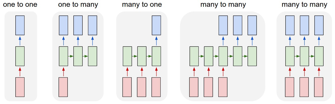
Today, we wil use a recurrent neural network. We will treat each tweet as a sequence of words. Like before, we will use GloVe embeddings as inputs to the recurrent network. (As a sidenote, not all recurrent neural networks use word embeddings as input. If we had a small enough vocabulary, we could have used a one-hot embedding of the words.)
import csv
import torch
import torch.nn as nn
import torch.nn.functional as F
import torch.optim as optim
import torchtext
import numpy as np
import matplotlib.pyplot as plt

def get_data():
    return csv.reader(open("training.1600000.processed.noemoticon.csv", "rt", encoding="latin-1"))

def split_tweet(tweet):
    # separate punctuations
    tweet = tweet.replace(".", " . ") \
                 .replace(",", " , ") \
                 .replace(";", " ; ") \
                 .replace("?", " ? ")
    return tweet.lower().split()

glove = torchtext.vocab.GloVe(name="6B", dim=50, max_vectors=10000) # use 10k most common words
Since we are going to store the individual words in a tweet, we will defer looking up the word embeddings. Instead, we will store the index of each word in a PyTorch tensor. Our choice is the most memory-efficient, since it takes fewer bits to store an integer index than a 50-dimensional vector or a word.
def get_tweet_words(glove_vector):
    train, valid, test = [], [], []
    for i, line in enumerate(get_data()):
        if i % 29 == 0:
            tweet = line[-1]
            idxs = [glove_vector.stoi[w]        # lookup the index of word
                    for w in split_tweet(tweet)
                    if w in glove_vector.stoi] # keep words that has an embedding
            if not idxs: # ignore tweets without any word with an embedding
                continue
            idxs = torch.tensor(idxs) # convert list to pytorch tensor
            label = torch.tensor(int(line[0] == "4")).long()
            if i % 5 < 3:
                train.append((idxs, label))
            elif i % 5 == 4:
                valid.append((idxs, label))
            else:
                test.append((idxs, label))
    return train, valid, test

train, valid, test = get_tweet_words(glove)
Here's what an element of the training set looks like:
tweet, label = train[0]
print(tweet)
print(label)
Unlike in the past, each element of the training set will have a different shape. The difference will present some difficulties when we discuss batching later on.
for i in range(10):
    tweet, label = train[i]
    print(tweet.shape)
Embedding
We are also going to use an nn.Embedding layer, instead of using the variable
glove directly. The reason is that the nn.Embedding layer lets us look up
the embeddings of multiple words simultaneously.
glove_emb = nn.Embedding.from_pretrained(glove.vectors)

# Example: we use the forward function of glove_emb to lookup the
# embedding of each word in `tweet`
tweet_emb = glove_emb(tweet)
tweet_emb.shape
Recurrent Neural Network Module
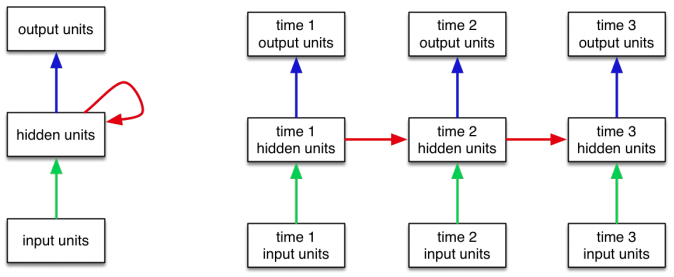
PyTorch has variations of recurrent neural network modules. These modules computes the following:
$$hidden = updatefn(hidden, input)$$ $$output = outputfn(hidden)$$
These modules are more complex and less intuitive than the usual neural network layers, so let's take a look:
rnn_layer = nn.RNN(input_size=50,    # dimension of the input repr
                   hidden_size=50,   # dimension of the hidden units
                   batch_first=True) # input format is [batch_size, seq_len, repr_dim]
Now, let's try and run this untrained rnn_layer on tweet_emb.
We will need to add an extra dimension to tweet_emb to account for
batching. We will also need to initialize a set of hidden units of size
[batch_size, 1, repr_dim], to be used for the first set of computations.
tweet_input = tweet_emb.unsqueeze(0) # add the batch_size dimension
h0 = torch.zeros(1, 1, 50)           # initial hidden state
out, last_hidden = rnn_layer(tweet_input, h0)
We don't technically have to explictly provide the initial hidden state, if we want to use an initial state of zeros. Just for today, we will be explicit about the hidden states that we provide.
out2, last_hidden2 = rnn_layer(tweet_input)
Now, let's look at the output and hidden dimensions that we have:
print(out.shape)
print(last_hidden.shape)
The shape of the hidden units is the same as our initial h0.
The variable out, though, has the same shape as our input.
The variable contains the concatenation of all of the output units
for each word (i.e. at each time point).
Normally, we only care about the output at the final time point, which we can extract like this.
out[:,-1,:]
This tensor summarizes the entire tweet, and can be used as an input to a classifier.
Building a Model
Let's put both the embedding layer, the RNN and the classifier into one model:
class TweetRNN(nn.Module):
    def __init__(self, input_size, hidden_size, num_classes):
        super(TweetRNN, self).__init__()
        self.emb = nn.Embedding.from_pretrained(glove.vectors)
        self.hidden_size = hidden_size
        self.rnn = nn.RNN(input_size, hidden_size, batch_first=True)
        self.fc = nn.Linear(hidden_size, num_classes)

    def forward(self, x):
        # Look up the embedding
        x = self.emb(x)
        # Set an initial hidden state
        h0 = torch.zeros(1, x.size(0), self.hidden_size)
        # Forward propagate the RNN
        out, _ = self.rnn(x, h0)
        # Pass the output of the last time step to the classifier
        out = self.fc(out[:, -1, :])
        return out

model = TweetRNN(50, 50, 2)
Now, this model has a very similar API as the previous. We should be able to train this model similar to any other model that we have trained before. However, there is one caveat that we have been avoiding this entire time, batching.
Batching
Unfortunately, we will not be able to use DataLoader with a
batch_size of greater than one. This is because each tweet has
a different shaped tensor.
for i in range(10):
    tweet, label = train[i]
    print(tweet.shape)
PyTorch implementation of DataLoader class expects all data samples
to have the same shape. So, if we create a DataLoader like below,
it will throw an error when we try to iterate over its elements.
#will_fail = torch.utils.data.DataLoader(train, batch_size=128)
#for elt in will_fail:
#    print("ok")
So, we will need a different way of batching.
One strategy is to pad shorter sequences with zero inputs, so that every sequence is the same length. The following PyTorch utilities are helpful.
torch.nn.utils.rnn.pad_sequencetorch.nn.utils.rnn.pad_packed_sequencetorch.nn.utils.rnn.pack_sequencetorch.nn.utils.rnn.pack_padded_sequence
(Actually, there are more powerful helpers in the torchtext module
that we will use in Lab 5. We'll stick to these in this demo, so that
you can see what's actually going on under the hood.)
from torch.nn.utils.rnn import pad_sequence

tweet_padded = pad_sequence([tweet for tweet, label in train[:10]],
                            batch_first=True)
tweet_padded.shape
Now, we can pass multiple tweets in a batch through the RNN at once!
out = model(tweet_padded)
out.shape
One issue we overlooked was that in our TweetRNN model, we always
take the last output unit as input to the final classifier. Now
that we are padding the input sequences, we should really be using
the output at a previous time step. Recurrent neural networks therefore
require much more record keeping than MLPs or even CNNs.
There is yet another problem: the longest tweet has many, many more words than the shortest. Padding tweets so that every tweet has the same length as the longest tweet is impractical. Padding tweets in a mini-batch, however, is much more reasonable.
In practice, practitioners will batch together tweets with the same length. For simplicity, we will do the same. We will implement a (more or less) straightforward way to batch tweets. Our implementation will be flawed, and we will discuss these flaws.
import random

class TweetBatcher:
    def __init__(self, tweets, batch_size=32, drop_last=False):
        # store tweets by length
        self.tweets_by_length = {}
        for words, label in tweets:
            # compute the length of the tweet
            wlen = words.shape[0]
            # put the tweet in the correct key inside self.tweet_by_length
            if wlen not in self.tweets_by_length:
                self.tweets_by_length[wlen] = []
            self.tweets_by_length[wlen].append((words, label),)

        #  create a DataLoader for each set of tweets of the same length
        self.loaders = {wlen : torch.utils.data.DataLoader(
                                    tweets,
                                    batch_size=batch_size,
                                    shuffle=True,
                                    drop_last=drop_last) # omit last batch if smaller than batch_size
            for wlen, tweets in self.tweets_by_length.items()}

    def __iter__(self): # called by Python to create an iterator
        # make an iterator for every tweet length
        iters = [iter(loader) for loader in self.loaders.values()]
        while iters:
            # pick an iterator (a length)
            im = random.choice(iters)
            try:
                yield next(im)
            except StopIteration:
                # no more elements in the iterator, remove it
                iters.remove(im)
Let's take a look at our batcher in action. We will set drop_last to be true for training,
so that all of our batches have exactly the same size.
for i, (tweets, labels) in enumerate(TweetBatcher(train, drop_last=True)):
    if i > 5: break
    print(tweets.shape, labels.shape)
Just to verify that our batching is reasonable, here is a modification of the
get_accuracy function we wrote last time.
def get_accuracy(model, data_loader):
    correct, total = 0, 0
    for tweets, labels in data_loader:
        output = model(tweets)
        pred = output.max(1, keepdim=True)[1]
        correct += pred.eq(labels.view_as(pred)).sum().item()
        total += labels.shape[0]
    return correct / total

test_loader = TweetBatcher(test, batch_size=64, drop_last=False)
get_accuracy(model, test_loader)
Our training code will also be very similar to the code we wrote last time:
def train_rnn_network(model, train, valid, num_epochs=5, learning_rate=1e-5):
    criterion = nn.CrossEntropyLoss()
    optimizer = torch.optim.Adam(model.parameters(), lr=learning_rate)
    losses, train_acc, valid_acc = [], [], []
    epochs = []
    for epoch in range(num_epochs):
        for tweets, labels in train:
            optimizer.zero_grad()
            pred = model(tweets)
            loss = criterion(pred, labels)
            loss.backward()
            optimizer.step()
        losses.append(float(loss))

        epochs.append(epoch)
        train_acc.append(get_accuracy(model, train_loader))
        valid_acc.append(get_accuracy(model, valid_loader))
        print("Epoch %d; Loss %f; Train Acc %f; Val Acc %f" % (
              epoch+1, loss, train_acc[-1], valid_acc[-1]))
    # plotting
    plt.title("Training Curve")
    plt.plot(losses, label="Train")
    plt.xlabel("Epoch")
    plt.ylabel("Loss")
    plt.show()

    plt.title("Training Curve")
    plt.plot(epochs, train_acc, label="Train")
    plt.plot(epochs, valid_acc, label="Validation")
    plt.xlabel("Epoch")
    plt.ylabel("Accuracy")
    plt.legend(loc='best')
    plt.show()
Let's train our model. Note that there will be some inaccuracies in computing the training loss.
We are dropping some data from the training set by setting drop_last=True. Again, the choice is
not ideal, but simplifies our code.
model = TweetRNN(50, 50, 2)
train_loader = TweetBatcher(train, batch_size=64, drop_last=True)
valid_loader = TweetBatcher(valid, batch_size=64, drop_last=False)
train_rnn_network(model, train_loader, valid_loader, num_epochs=20, learning_rate=2e-4)
get_accuracy(model, test_loader)


The hidden size and the input embedding size don't have to be the same.
#model = TweetRNN(50, 100, 2)
#train_rnn_network(model, train_loader, valid_loader, num_epochs=80, learning_rate=2e-4)
#get_accuracy(model, test_loader)
LSTM for Long-Term Dependencies
There are variations of recurrent neural networks that are more powerful. One such variation is the Long Short-Term Memory (LSTM) module. An LSTM is like a more powerful version of an RNN that is better at perpetuating long-term dependencies. Instead of having only one hidden state, an LSTM keeps track of both a hidden state and a cell state.
lstm_layer = nn.LSTM(input_size=50,   # dimension of the input repr
                    hidden_size=50,   # dimension of the hidden units
                    batch_first=True) # input format is [batch_size, seq_len, repr_dim]
Remember the single tweet that we worked with earlier?
tweet_emb.shape
This is how we can feed this tweet into the LSTM, similar to what we tried with the RNN earlier.
tweet_input = tweet_emb.unsqueeze(0) # add the batch_size dimension
h0 = torch.zeros(1, 1, 50)     # initial hidden layer
c0 = torch.zeros(1, 1, 50)     # initial cell state
out, last_hidden = lstm_layer(tweet_input, (h0, c0))
out.shape
So an LSTM version of our model would look like this:
class TweetLSTM(nn.Module):
    def __init__(self, input_size, hidden_size, num_classes):
        super(TweetLSTM, self).__init__()
        self.emb = nn.Embedding.from_pretrained(glove.vectors)
        self.hidden_size = hidden_size
        self.rnn = nn.LSTM(input_size, hidden_size, batch_first=True)
        self.fc = nn.Linear(hidden_size, num_classes)

    def forward(self, x):
        # Look up the embedding
        x = self.emb(x)
        # Set an initial hidden state and cell state
        h0 = torch.zeros(1, x.size(0), self.hidden_size)
        c0 = torch.zeros(1, x.size(0), self.hidden_size)
        # Forward propagate the LSTM
        out, _ = self.rnn(x, (h0, c0))
        # Pass the output of the last time step to the classifier
        out = self.fc(out[:, -1, :])
        return out

model_lstm = TweetLSTM(50, 50, 2)
train_rnn_network(model, train_loader, valid_loader, num_epochs=20, learning_rate=2e-5)
get_accuracy(model, test_loader)


GRU for Long-Term Dependencies
Another variation of an RNN is the Gated-Recurrent Unit (GRU). The GRU is invented after LSTM, and is intended to be a simplification of the LSTM that is still just as powerful. The nice thing about GRU units is that they have only one hidden state.
gru_layer = nn.GRU(input_size=50,   # dimension of the input repr
                   hidden_size=50,   # dimension of the hidden units
                   batch_first=True) # input format is [batch_size, seq_len, repr_dim]
The GRU API is virtually identical to that of the vanilla RNN:
tweet_input = tweet_emb.unsqueeze(0) # add the batch_size dimension
h0 = torch.zeros(1, 1, 50)     # initial hidden layer
out, last_hidden = gru_layer(tweet_input, h0)
out.shape
So a GRU version of our model would look similar to before:
class TweetGRU(nn.Module):
    def __init__(self, input_size, hidden_size, num_classes):
        super(TweetGRU, self).__init__()
        self.emb = nn.Embedding.from_pretrained(glove.vectors)
        self.hidden_size = hidden_size
        self.rnn = nn.GRU(input_size, hidden_size, batch_first=True)
        self.fc = nn.Linear(hidden_size, num_classes)

    def forward(self, x):
        # Look up the embedding
        x = self.emb(x)
        # Set an initial hidden state
        h0 = torch.zeros(1, x.size(0), self.hidden_size)
        # Forward propagate the GRU
        out, _ = self.rnn(x, h0)
        # Pass the output of the last time step to the classifier
        out = self.fc(out[:, -1, :])
        return out

model_lstm = TweetGRU(50, 50, 2)
train_rnn_network(model, train_loader, valid_loader, num_epochs=20, learning_rate=2e-5)
get_accuracy(model, test_loader)

