Convolutional Neural Networks
So far, we have used feed-forward neural networks with fully connected layers to build neural networks. While fully connected layers are useful, they also have undesirable properties.
Specifically, fully connected layers require a lot of connections, and thus many more weights than our problem might need. Suppose we are trying to determine whether a greyscale image of size $200 \times 200$ contains a cat. Our input layer would have $200 \times 200 = 40000$ units: one for each pixel. A fully connected layer between the input and the first hidden layer with, say, 500 hidden units will require at least $40000 \times 500 =$ 20 million weights!
The large number of weights mean several things. First, computing predictions will require long processing time. Second, our network very high capacity, and will be prone to overfitting. We will need a large number of training examples, or be very aggressive in preventing overfitting (we'll discuss some techniques in a later lecture).
There are other undesirable properties as well. What happens if our input image is shifted by one pixel to the left? Since the content of the image is virtually unchanged, we would like our prediction to change very little as well. However, each pixel is now being multiplied by an entirely different neural network weight. We could get a completely different prediction. In short, a fully-connected layer does not explicitly take the 2D geometry of the image into consideration.
In this chapter, we will introduce the convolutional neural network to solve many of these aforementioned issues.
Locally Connected Layers
In a 2-dimensional images, there is a notion of proximity. If you want to know what object is at at a particular pixel, you can usually find out by looking at other pixels nearby. (At the very list, nearby pixels will be more informative than pixels further away.) In fact, many features that the human eye can easily detect are local features. For example, we can detect edges, textures, and even shapes using pixel intensities in a small region of an image.
If we want a neural network to detect these kinds of local features, we can use a locally connected layer, like this:
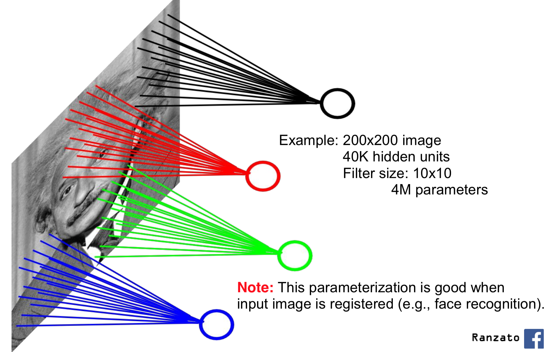
Each unit in the (first) hidden layer detects patterns in a small portion of the input image, rather than the entire image. This way, we have fewer connections (and therefore weights) between the input and the first hidden layer. Note that now, the hidden layers will also have a geometry to them, with the top-left corner of the hidden layers being computed from the top-left region of the original input image.
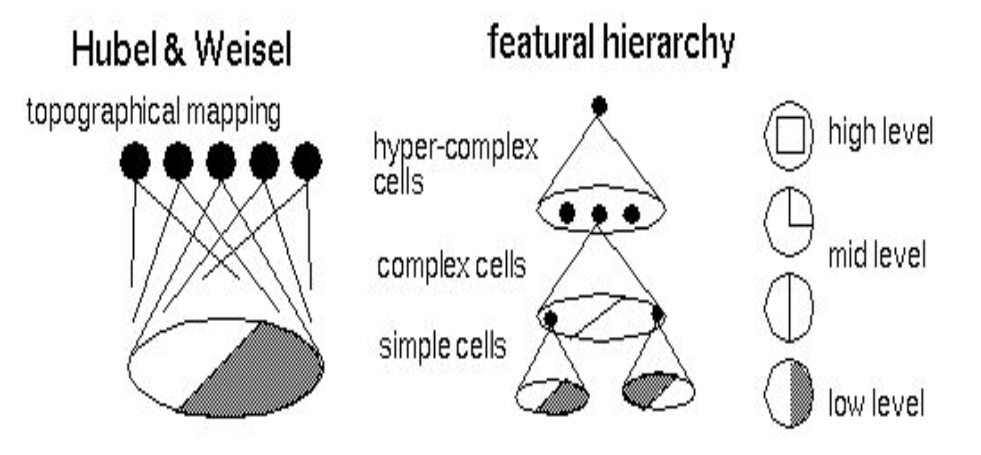
There is actually evidence that the (biological) neural connectivity in an animal's visual cortex works similarly. That is, neurons in the visual cortex detect features that occur in a small region of our receptive field. Neurons close to the retina detect simple patterns like edges. Neurons that receive information from these simple cells detect more complicated patterns, like textures and blobs. Neurons in even higher layers detect even more complicated patterns, like entire hands or faces.
Weight Sharing
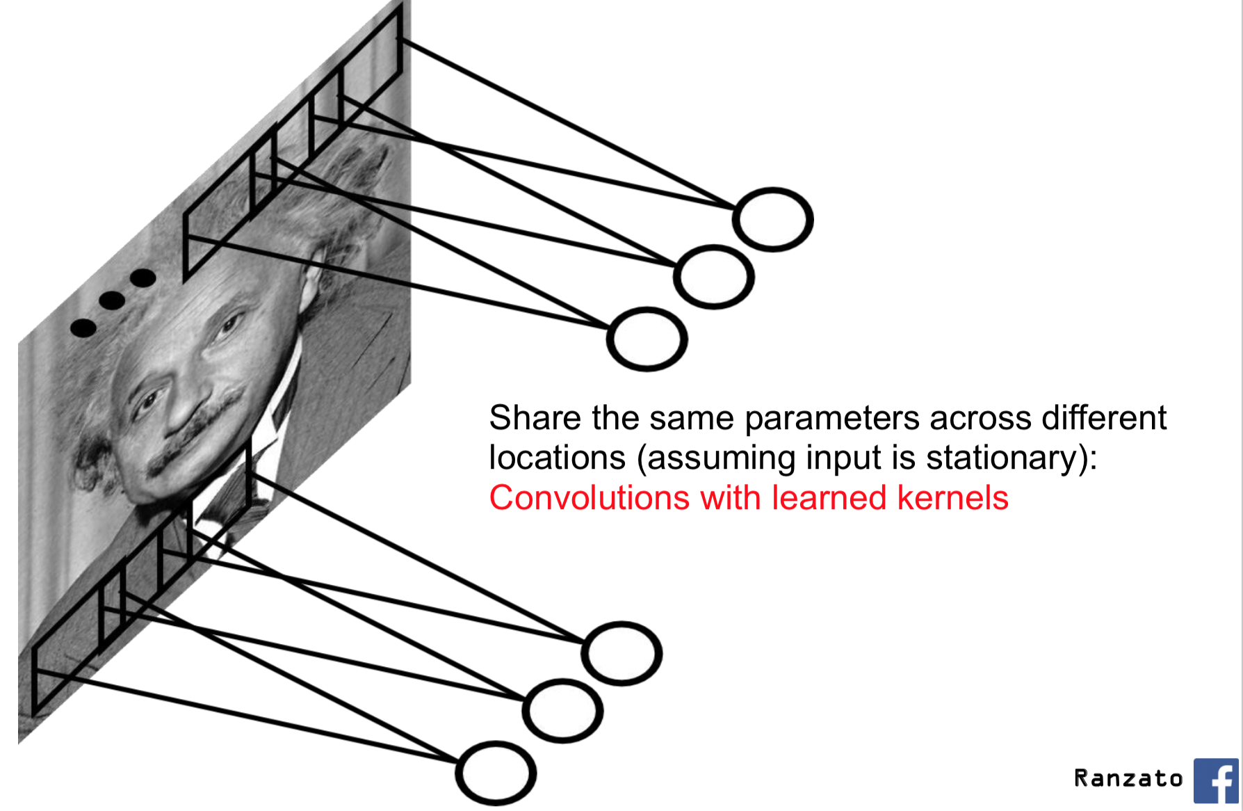
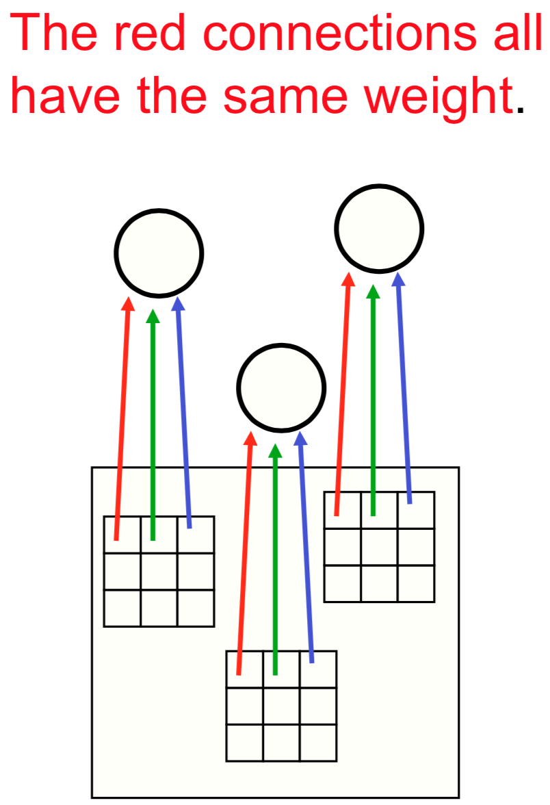
Besides restricting ourselves to only local connections, there is one other optimization we can make: if we wanted to detect a feature (say, a horizontal edge), we can use the same detector on the bottom-left corner of an image and on the top right of the image. That is, if we know how to detect a local feature in one region of the image, then we know how to detect that feature in all other regions of the image. In neural networks, "knowing how to detect a local feature" means having the appropriate weights and biases connecting the input neurons to some hidden neuron.
We can therefore reuse the same weights everywhere else in the image. This is the idea behind weight sharing: we will share the same parameters across different locations in an image.
Convolutional Arithmetic (forward pass computation)
Let's look at the forward pass computation of a convolutional neural network layer. That is, let's pretend to be PyTorch and compute the output of a convolutional layer, given some input.
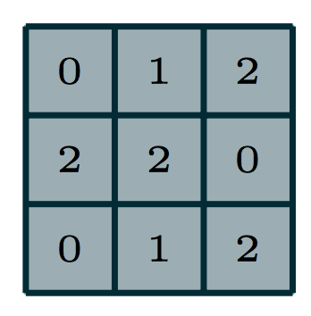
The light blue grid (middle) is the input that we are given. You can imagine that this blue grid represents a 5 pixel by 5 pixel greyscale image.
The grey grid (left) contains the parameters of this neural network layer. This grey grid is also known as a convolutional kernel, convolutional filter, or just kernel or filter. In this case, the kernel size or filter size is $3 \times 3$.
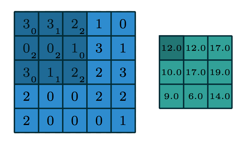
To compute the output, we superimpose the kernel on a region of the image. Let's start at the top left, in the dark blue region. The small numbers in the bottom right corner of each grid element corresponds to the number in the kernel. To compute the output at the corresponding location (top left), we "dot" the pixel intensities in the square region with the kernel. That is, we perform the computation:
(3 * 0 + 3 * 1 + 2 * 2) + (0 * 2 + 0 * 2 + 1 * 0) + (3 * 0 + 1 * 1 + 2 * 2)
The green grid (right) contains the output of this convolution layer. This output is also called an output feature map. The terms feature, and activation are interchangable. The output value on the top left of the green grid is consistent with the value we obtained by hand in Python.
To compute the next activation value (say, one to the right of the previous output), we will shfit the superimposed kernel over by one pixel:
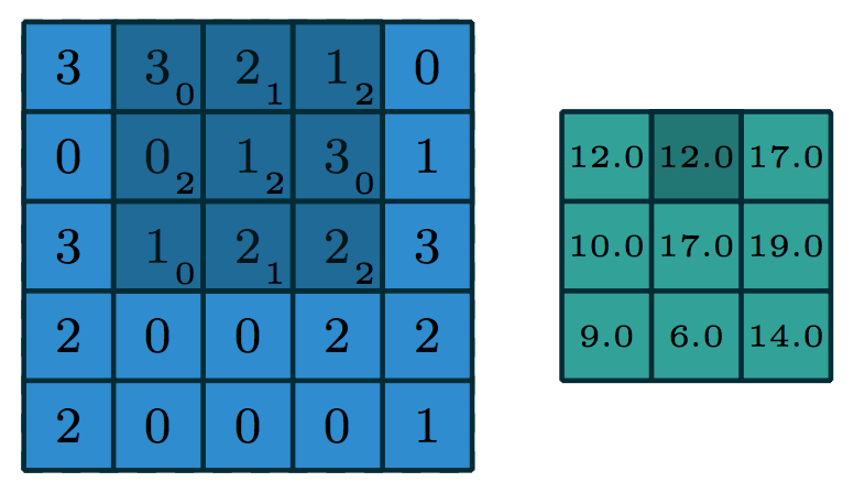
The dark blue region is moved to the right by one pixel. We again dot the pixel intensities in this region with the kernel:
(3 * 0 + 2 * 1 + 1 * 2) + (0 * 2 + 1 * 2 + 3 * 0) + (1 * 0 + 2 * 1 + 2 * 2)
And the pattern continues...
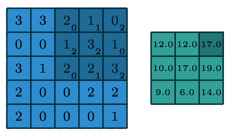
(2 * 0 + 1 * 1 + 0 * 2) + (1 * 2 + 3 * 2 + 1 * 0) + (2 * 0 + 2 * 1 + 3 * 2)
One part of the computation that is missing in this picture is the addition of a bias term, which we will discuss later.
Filters in Computer Vision
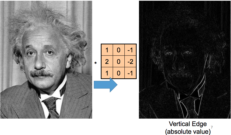
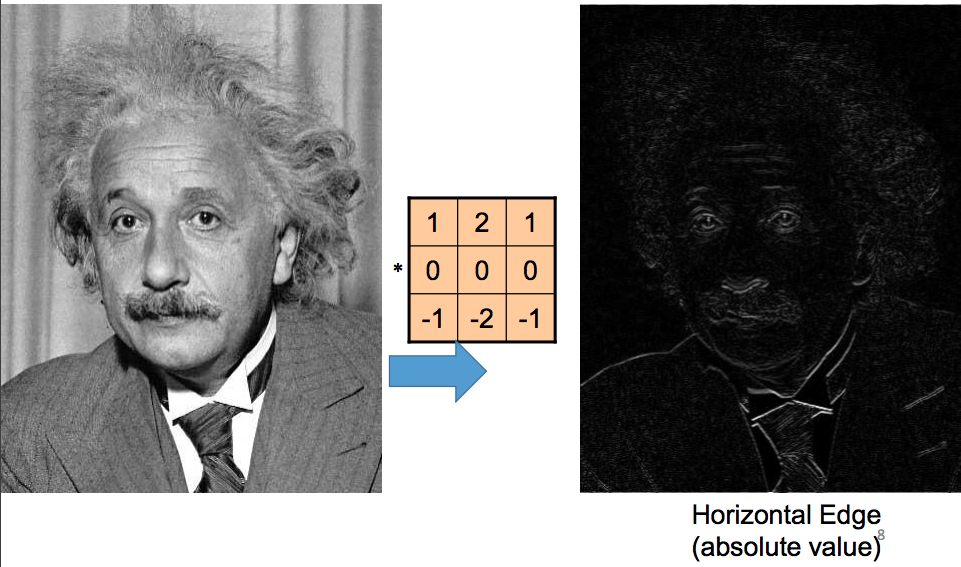
Are filters actually useful? Can we use filters to detect a variety of useful features? The answer is yes! In fact, people have used the idea of convolutional filters in computer vision even before the rise of machine learning. They hand-coded filters that can detect simple features, for example to detect edges in various orientations:
Convolutions with Multiple Input/Output Channels
There are two more things we might want out of the convolution operation.
First, what if we were working with a colour image instead of a greyscale image? In that case, the kernel will be a 3-dimensional tensor instead of a 2-dimensional one. This kernel will move through the input features just like before, and we "dot" the pixel intensities with the kernel at each region, exactly like before:
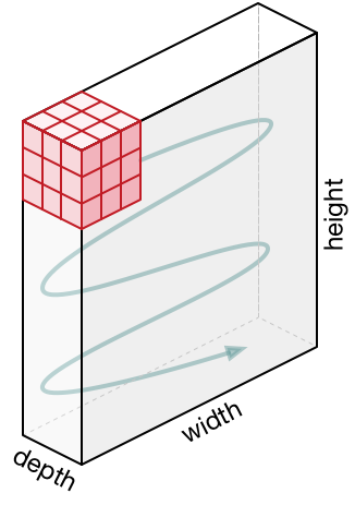
In case of an RGB image, the size of the new dimension (aside from the width/height of the image) is 3. This "size of the 3rd dimension" is called the number of input channels or number of input feature maps. In the above image example, the number of input channels is 3, and we have a $3 \times 3 \times 3$ kernel.
Second, what if we want to detect multiple features? For example, we may wish to detect both horizontal edges and vertical edges, or any other learned features? We would want to learn many convolutional filters on the same input. That is, we would want to make the same computation above using different kernels, like this:
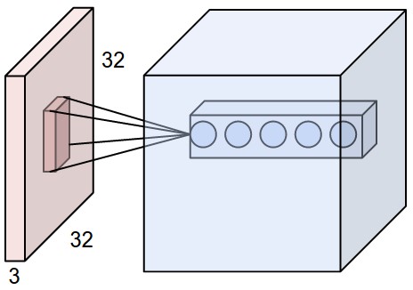
Each circle on the right of the image represents the output of a different kernel dotted with the highlighted region on the right. So, the output feature is also a 3-dimensional tensor. The size of the new dimension is called the number of output channels or number of output feature maps. In the picture above, there are 5 output channels.
The Convolutional Layers in PyTorch
Finally, let's create convolutional layers in PyTorch!
Recall that in PyTorch, we can create a fully-connected layer between successive layers like this:
%matplotlib inline
import torch.nn as nn

# fully-connected layer between a lower layer of size 100, and
# a higher layer of size 30
fc = nn.Linear(100, 30)
We've applied a layer like this as follows:
import torch
x = torch.randn(100) # create a tensor of shape [100]
y = fc(x)            # apply the fully conected layer `fc` to x
y.shape
We will be examining the <Tensor>.shape attribute a lot today to help
us ensure that we truly understand what is going on. If we understood,
for example, what the layer fc does, we should have been able to predict
the shape of y before running the above code.
In PyTorch, we can create a convolutional layer using nn.Conv2d:
conv = nn.Conv2d(in_channels=3,  # number of input channels
                 out_channels=7, # number of output channels
                 kernel_size=5)  # size of the kernel
The conv layer expects as input a tensor in the format "NCHW", meaning that
the dimensions of the tensor should follow the order:
- batch size
- channel
- height
- width
For example, we can emulate a batch of 32 colour images, each of size 128x128, like this:
x = torch.randn(32, 3, 128, 128)
y = conv(x)
y.shape
The output tensor is also in the "NCHW" format. We still have 32 images, and 7 channels
(consistent with out_channels of conv), and of size 124x124. If we added the appropriate
padding to conv, namely padding = kernel_size // 2, then our output width and height should
be consistent with the input width and height:
conv2 = nn.Conv2d(in_channels=3,
                  out_channels=7,
                  kernel_size=5,
                  padding=2)

x = torch.randn(32, 3, 128, 128)
y = conv2(x)
y.shape
To further illustrate the formatting, let's apply the (random, untrained) convolution conv2 to
a real image. First, we load the image:
import matplotlib.pyplot as plt
import numpy as np

img = plt.imread("imgs/dog_mochi.png")[:, :, :3]
plt.imshow(img)

Then, we convert the image into a PyTorch tensor of the appropriate shape.
x = torch.from_numpy(img) # turn img into a PyTorch tensor
print(x.shape)
x = x.permute(2,0,1)      # move the channel dimension to the beginning
print(x.shape)
x = x.reshape([1, 3, 350, 210]) # add a dimension for batching
print(x.shape)
Even when our batch size is 1, we still need the first dimension so that the input follows the "NCHW" format.
y = conv2(x)           # apply the convolution
y = y.detach().numpy() # convert the result into numpy
y = y[0]               # remove the dimension for batching

# normalize the result to [0, 1] for plotting
y_max = np.max(y)
y_min = np.min(y)
img_after_conv = y - y_min / (y_max - y_min)
img_after_conv.shape
Let's plot the 7 channels one by one:
plt.figure(figsize=(14,4))
for i in range(7):
    plt.subplot(1, 7, i+1)
    plt.imshow(img_after_conv[i])

If we were to run a neural network, these would be the unit outputs (prior to applying the activation function).
Parameters of a Convolutional Layer
Recall that the trainable parameters of a fully-connected layer includes the network weights and biases. There is one weight for each connection, and one bias for each output unit:
fc = nn.Linear(100, 30)
fc_params = list(fc.parameters())
print("len(fc_params)", len(fc_params))
print("Weights:", fc_params[0].shape)
print("Biases:", fc_params[1].shape)
In a convolutional layer, the trainable parameters include the convolutional kernels (filters) and also a set of biases:
conv2 = nn.Conv2d(in_channels=3,
                  out_channels=7,
                  kernel_size=5,
                  padding=2)
conv_params = list(conv2.parameters())
print("len(conv_params):", len(conv_params))
print("Filters:", conv_params[0].shape)
print("Biases:", conv_params[1].shape)
There is one bias for each output channel. Each bias is added to every element in that output channel. Note that the bias computation was not shown in the above figures, and are often omitted in other texts describing convolutional arithmetics. Nevertheless, the biases are there.
Pooling Layers
A pooling layer can be created like this:
pool = nn.MaxPool2d(kernel_size=2, stride=2)
y = conv2(x)
z = pool(y)
z.shape
Usually, the kernel size and the stride length will be equal.
The pooling layer has no trainable parameters:
list(pool.parameters())
Convolutional Networks in PyTorch
In assignment 2, we created the following network. We can understand this network now!
class LargeNet(nn.Module):
    def __init__(self):
        super(LargeNet, self).__init__()
        self.name = "large"
        self.conv1 = nn.Conv2d(3, 5, 5)
        self.pool = nn.MaxPool2d(2, 2)
        self.conv2 = nn.Conv2d(5, 10, 5)
        self.fc1 = nn.Linear(10 * 5 * 5, 32)
        self.fc2 = nn.Linear(32, 1)

    def forward(self, x):
        x = self.pool(F.relu(self.conv1(x)))
        x = self.pool(F.relu(self.conv2(x)))
        x = x.view(-1, 10 * 5 * 5)
        x = F.relu(self.fc1(x))
        x = self.fc2(x)
        x = x.squeeze(1) # Flatten to [batch_size]
        return x
This network has two convolutional layers: conv1 and conv2.
- The first convolutional layer
conv1requires an input with 3 channels, outputs 5 channels, and has a kernel size of5x5. We are not adding any zero-padding. - The second convolutional layer
conv1requires an input with 5 channels, outputs 10 channels, and has a kernel size of (again)5x5. We are not adding any zero-padding.
In the forward function we see that the convolution operations are always
followed by the usual ReLU activation function, and a pooling operation.
The pooling operation used is max pooling, so each pooling operation
reduces the width and height of the neurons in the layer by half.
Because we are not adding any zero padding, we end up with 10 * 5 * 5 hidden units
after the second convolutional layer. These units are then passed to two fully-connected
layers, with the usual ReLU activation in between.
Notice that the number of channels grew in later convolutional layers! However, the number of hidden units in each layer is still reduced because of the pooling operation:
- Initial Image Size: $3 \times 32 \times 32 = 3072$
- After
conv1: $5 \times 28 \times 28$ - After Pooling: $5 \times 14 \times 14 = 980$
- After
conv2: $10 \times 10 \times 10$ - After Pooling: $10 \times 5 \times 5 = 250$
- After
fc1: $32$ - After
fc2: $1$
This pattern of doubling the number of channels with every pooling / strided convolution is common in modern convolutional architectures. It is used to avoid loss of too much information within a single reduction in resolution.
AlexNet in PyTorch
Convolutional networks are very commonly used, meaning that there are often alternatives to training convolutional networks from scratch. In particular, researchers often release both the architecture and the weights of the networks they train.
As an example, let's look at the AlexNet model, whose trained weights are included in torchvision.
AlexNet was trained to classify images into one of many categories.
The AlexNet can be imported like below.
import torchvision.models

alexNet = torchvision.models.alexnet(pretrained=True)
alexNet
Notice that the AlexNet model is split into two parts. There is a component that computes "features" using convolutions.
alexNet.features
There is also a component that classifies the image based on the computed features.
alexNet.classifier
AlexNet Features
The first network can be used independently of the second. Specifically, it can be used to compute a set of features that can be used later on. This idea of using neural network activation features to represent images is an extremely important one, so it is important to understand the idea now.
If we take our image x from earlier and apply it to the alexNet.features network,
we get some numbers like this:
features = alexNet.features(x)
features.shape
The set of numbers in features is another way of representing our image x. Recall that
our initial image x was also represented as a tensor, also a set of numbers representing
pixel intensity. Geometrically speaking, we are using points in a high-dimensional space to
represent the images. in our pixel representation, the axes in this high-dimensional space
were different pixels. In our features representation, the axes are not as easily
interpretable.
But we will want to work with the features representation, because this representation
makes classification easier. This representation organizes images in a more "useful" and
"semantic" way than pixels.
Let me be more specific:
this set of features was trained on image classification. It turns out that
these features can be useful for performing other image-related tasks as well!
That is, if we want to perform an image classification task of our own (for example,
classifying cancer biopsies, which is nothing like what AlexNet was trained to do),
we might compute these AlexNet features, and then train a small model on top of those
features. We replace the classifier portion of AlexNet, but keep its features
portion intact.
Somehow, through being trained on one type of image classification problem, AlexNet learned something general about representing images for the purposes of other classification tasks.
AlexNet First Convolutions
Since we have a trained model, we might as well visualize outputs of a trained convolution, to contrast with the untrained convolution we visualized earlier.
Here is the first convolution of AlexNet, applied to our image of Mochi.
alexNetConv = alexNet.features[0]
y = alexNetConv(x)
The output is a $1 \times 64 \times 86 \times 51$ tensor.
y = y.detach().numpy()
y = (y - y.min()) / (y.max() - y.min())
y.shape
We can visualize each channel independently.
plt.figure(figsize=(10,10))
for i in range(64):
    plt.subplot(8, 8, i+1)
    plt.imshow(y[0, i])
