From Pigeons to Artificial Neural Networks
Artificial neural networks draw inspiration from real neural networks. In order to understand deep learning using a "top-down" approach, we'll start with a familiar system capable of learning: a pigeon.
In 2015, researchers Levenson et al. from the University of California Davis trained pigeons to detect breast cancer. They show that the common pigeon can reliably distinguish between benign versus malignant tumors. The experimental setup is shown below.
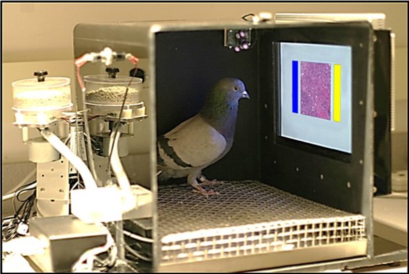
The researchers trained pigeons by showing an image of a magnified biopsy to a pigeon. The pigeon then pecks at one of two answer buttons, labelling the image as malignant (cancerous) or benign (not cancerous). If the pigeon chooses correctly, researchers reward it with a tasty food pellet.
You can imagine that at the very beginning, the pigeons might peck randomly, perhaps not even pecking at the buttons at all. Eventually, the pigeon might accidentally peck at the correct button, and see a food pellet. This food pellet is extremely important, and is what guides the pigeon to change its behaviour.
In a sense, training an artificial neural network is like training a pigeon. In both cases, we need to answer questions like:
- How will we reward the pigeon (neural network)?
- How do we train the pigeon (neural network) quickly and efficiently?
- How do we know that the pigeon (neural network) did not just memorize the pictures we show it?
- Are there ethical issues in trusting a pigeon (neural network) to detect cancer?
In this chapter, we'll build an artificial pigeon instead of using a real one. Also, instead of using pigeons to detect cancer, we'll work on a simpler problem of categorizing digits. In order to use an artificial pigeon to solve our classification problem, we will need to:
- Build an artificial pigeon -- or rather, an artificial pigeon brain
- Decide how to reward the artificial pigeon
- Decide how to train the artificial pigeon
- Determine how well our artificial pigeon performs the classification task
We will look at each problem in turn.
The Pigeon Brain
How does a pigeon "work"? How were pigeons able to link the visual features of the biopsy images to receiving the food pellets? We don't know everything about how pigeons work, but we do know this much:
- The light emitted from the screen showing the biopsy images reaches the pigeon's retina.
- Each retinal cell sends signals to neurons attached to it.
- The neurons pass the information to other neurons that are a part of the bird's brain.
- The brain makes a decision about what action to take.
- Neurons send signals to various parts of the pigeon's body, which results in the pigeon pecking a button (or not).
- The pigeon observes the response of its environment. Its neural pathways and biochemistry change to adapt to the environment.
Much of these steps remain a mystery as of early 2019. However, we do know a few things about how biological neurons work, and we will use that knowledge to build a mathematical model of an artificial neuron.
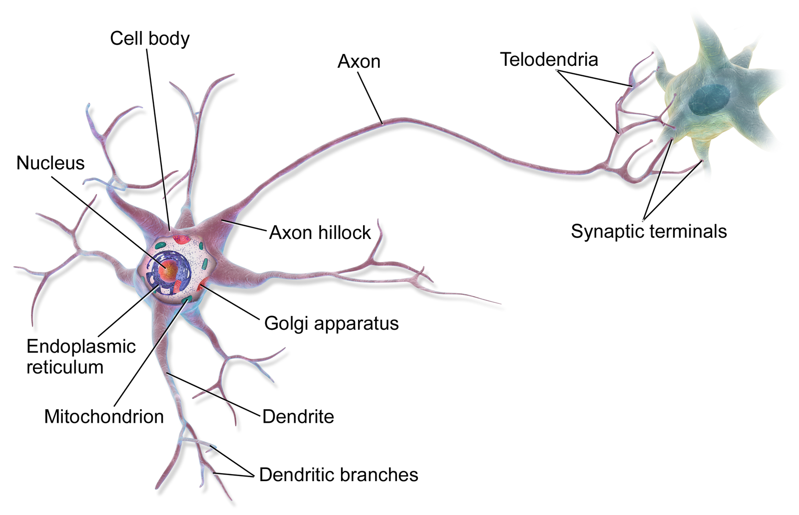
The figure above shows the anatomy of a brain cell, called a neuron. For our purposes, the most important parts of the neuron are:
- The dendrites, which are connected to other cells that provides information.
- The cell body, which consolidates information from the dendrites.
- The axon, which is an extension from the cell body that passes information to other cells.
- The synapse, which is the area where the axon of one neuron and the dendrite of another connect.
Neurons pass information using action potentials. When a neuron is "at rest", there is a small voltage difference between the inside and outside of the cell. When a neuron receives "information" in its dendrites, the voltage difference along that part of the cell lowers. If the total activity in a neuron's dendrites lowers the voltage difference enough, the entire cell depolarizes. In other words, the neuron fires. The voltage signal spreads along the axon and to the synapse, then to the next cells. Depending on the total activity at the next cells' dendrites, the signal might continue to propagate.
What does it mean when a particular neuron fires? This question, known as neural decoding, is very difficult to answer. However, neuroscientists do know that cells in the optic pathway fire more in response to various visual stimuli. There are neurons that fire more when a particular retinal cell is excited. There are also neurons that fire more in response to specific edges, lines, angles, and movements. There are neurons in monkeys that fire selectively to hands and faces. In 2005, studies found evidence of cells that fire in response to particular people like Bill Clinton or Jennifer Aniston. These studies lead to the hypothesis of a "grandmother cell", a neuron that represents a complex but specific concept or object.
The existence of such "grandmother cells" is still contested. Many believe that neuron firing patterns encode information only in a distributed fashion. That is, the firing of a single neuron does not have a particular meaning, but the firing pattern of a group of neurons do. The idea is akin to how if you look at the bit patterns of an encrypted file, the individual bit values mean very little on their own, without considerations of other bits in the file.
An Artificial Pigeon Brain
For the purpose of modelling an artificial brain, we will make make the simplifying assumption that a "grandmother cell" exists. This cell is the output of our network, representing the prediction we wish to make. That is, if we are hoping to classify malignant vs benign biopsy scans, we will have an output neuron that will (hopefully) only fire in the presence of a malignant tumor, not a benign one. Our goal when training this artificial neural network is to make this output neuron behave the way we want.
We will also need to model neurons that read the input. In a biological brain, there are neurons that connect directly to retinal cells and activate when those cells activate. For our purposes, we will also have input neurons, one for each pixel in the image.
The input neurons need to be connected to the output in some way. In a biological brain, the connections between neurons are messy, and can contain loops. In our case, we will use a "feed-forward" network with discrete layers, like this:
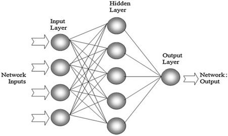
Each neuron will belong to a layer. In our case, there is an input layer, one hidden layer, and an output layer with a single output neuron. Each neuron will be connected to all neurons in the layers below and above. The hidden layer receives information from the input layer, and passes information the output layer. In theory, we can have more than one hidden layer. In fact, we can have as many hidden layers as we want. The more hidden layers we have, the deeper our network.
This "layered" neural network architecture is called a fully-connected, feed-forward network. It is fully-connected because neurons connect to all other neurons in the preceding and succeeding layer. It is feed-forward because information only flows in one direction: there is no information flow from a later layer back to an earlier layer. For historical reasons, this network architecture is also called a multi-layer perceptron (MLP).
We have still yet to model the individual neurons themselves. We will use real numbers to represent the firing rate of neurons, or the neuron's activation. We interpret a high activation value to mean a very active neuron, and a low activation value to mean an inactive neuron. The activation of the input neuron is set to the intensity of the corresponding pixel.
The degree to which a biological neuron's activation influences another is complex, and depends on the presence and absence of neurotransmitters, and other biochemical and biophysical factors. In our artificial neuron, we will summarize all those factors into one real number, called a weight. This number can be large or small, and can be positive or negative. The strength of connections between neurons will change and adjust during training.
So far, the activation of a neuron is a scaled sum of the activations of the neurons in the layer below. However, in a biological neuron, the total sum of activity in the dendrites needs to be above a threshold in order for the neuron to fire. We will model the (negative) threshold as another real value that we add (subtract) from the activation, and set all activation below zero to be zero. The threshold numbers, called biases, are different for each neuron, and will also change during training.
Here is an implementation of the artificial pigeon brain in PyTorch. Don't worry if this code or the explanations don't make sense yet.
import torch
import torch.nn as nn
import torch.nn.functional as F
import matplotlib.pyplot as plt # for plotting

torch.manual_seed(1) # set the random seed

class Pigeon(nn.Module):
    def __init__(self):
        super(Pigeon, self).__init__()
        self.layer1 = nn.Linear(28 * 28, 30)
        self.layer2 = nn.Linear(30, 1)
    def forward(self, img):
        flattened = img.view(-1, 28 * 28)
        activation1 = self.layer1(flattened)
        activation1 = F.relu(activation1)
        activation2 = self.layer2(activation1)
        return activation2

pigeon = Pigeon()
In this network, there are 28x28 = 784 input neurons, suggesting that our input image should be 28x28 pixels large. We have a single output neuron. We also have 30 neurons in the hidden layer.
The variable pigeon.layer1 contains information about the connectivity
between the input layer and the hidden layer (stored as a matrix), and the
hidden layer biases (stored as a vector).
Similarly, the variable pigeon.layer2 contains information about the weights
between the hidden layer and the output layer, and the output neuron's bias.
The weights and biases adjust during training, so they are called the model's
parameters.
We can introspect their values:
for w in pigeon.layer2.parameters():
    print(w)
Training
The weights that we see above were randomly initialized by PyTorch. Most likely, they are not suitable for whatever task we want the network to perform. So, we need to "train" the network: to adjust these weights (and biases) so that the network does do what we want.
Training is where our "pigeon analogy" falls apart. We posit that the biochemistry and connectivity of biological neurons can change based on past experience. However, the way that we train our artificial neural network bears no resemblance to the way pigeons and other animals might learn.
Here's what training will entail:
- We're going to ask our network to make a prediction for some input data, whose output we already know.
- We're going to compare the predict output to the ground truth, actual output.
- We're going to adjust the parameters to make the prediction closer to the ground truth. (This is the magic behind machine learning.)
- We'll repeat steps 1-3. (The question of when to stop is an interesting one, which we won't talk about yet.)
In order to train the network, we need a set of input data to which we know the desired output.
Digit Recognition
We will train this "artificial pigeon" to perform a digit recognition task. That is, we will use the MNIST dataset of hand-written digits, and train the pigeon to recognize a small digit, namely a digit that is less than 3. This problem is a binary classification problem we want to predict which of two classes an input image is a part of.
The MNIST dataset contains hand-written digits that are 28x28 pixels large. Here are a few digits in the dataset:
from torchvision import datasets, transforms

# load the training data
mnist_train = datasets.MNIST('data', train=True, download=True)
mnist_train = list(mnist_train)[:2000]

# plot the first 18 images in the training data
for k, (image, label) in enumerate(mnist_train[:18]):
    plt.subplot(3, 6, k+1)
    plt.imshow(image)

Here is an example of using the network to classify whether the last image contains a small digit. Again, since we haven't trained the network yet, the predicted probability of the image containing a small digit is close to half. The "pigeon" is unsure.
# transform the image data type to a 28x28 matrix of numbers
img_to_tensor = transforms.ToTensor()

inval = img_to_tensor(image)
outval = pigeon(inval)       # find the output activation given input
prob = torch.sigmoid(outval) # turn the activation into a probability
print(prob)
In fact, if we show the network different images, the predicted probabilities will be very similar, and will be around half.
for k, (image, label) in enumerate(mnist_train[:10]):
    print(torch.sigmoid(pigeon(img_to_tensor(image))))
In order for the network to be useful, we need to actually train it, so that the weights are actually meaningful, non-random values. As we mentioned before, we'll use the network to make predictions, then compare the predictions agains the ground truth. But how do we compare the predictions against the ground truth? We'll need a few more things. In particular, we need to:
- Specifying a "reward" or a loss (negative reward) that judges how good or bad the prediction was, compared to the ground truth actual value.
- Specifying an optimizer that tunes the parameters to improve the reward or loss.
Choosing a good loss function $L(actual, predicted)$ for a problem is not a trivial task. The definition of a loss function also transforms a classification problem into an optimization problem: what set of parameters minimizes the loss (or maximizes the reward) across the training examples?
Turning a learning problem into an optimization problem is actually a very subtle but important step in many machine learning tools, because it allows us to use tools from mathematical optimization.
That there are optimizers that can tune the network parameters for us is also really, really cool. Unfortunately, we won't talk much about optimizers and how they work in this course. You should know though that these optimizers are what makes machine learning work at all.
For now, we will choose a standard loss function for a binary classification problem: the binary cross-entropy loss. We'll also choose a stochastic gradient descent optimizer. We'll talk about what these mean later in the course.
import torch.optim as optim

criterion = nn.BCEWithLogitsLoss()
optimizer = optim.SGD(pigeon.parameters(), lr=0.005, momentum=0.9)
Now, we can start to train the pigeon network, similar to the way we would train a real pigeon:
- We'll show the network pictures of digits, one by one
- We'll see what the network predicts
- We'll check the loss function for that example digit, comparing the network prediction against the ground truth
- We'll make a small update to the parameters to try and improve the loss for that digit
- We'll continue doing this many times -- let's say 1000 times
For simplicity, we'll use 1000 images, and show the network each image only once.
# simplified training code to train `pigeon` on the "small digit recognition" task

for (image, label) in mnist_train[:1000]:
    # actual ground truth: is the digit less than 3?
    actual = (label < 3).reshape([1,1]).type(torch.FloatTensor)
    # pigeon prediction
    out = pigeon(img_to_tensor(image)) # step 1-2
    # update the parameters based on the loss
    loss = criterion(out, actual)      # step 3
    loss.backward()                    # step 4 (compute the updates for each parameter)
    optimizer.step()                   # step 4 (make the updates for each parameter)
    optimizer.zero_grad()              # a clean up step for PyTorch
Let's see how the pigeon performs on the last image it was trained on:
# display the last training image
plt.imshow(image)

Here's the predicted probability that the image is a small digit (less than 3).
inval = img_to_tensor(image)
outval = pigeon(img_to_tensor(image))
prob = torch.sigmoid(outval)
print(prob)
Here are some more predictions for some of the digits we plotted eariler:
# predictions for the first 10 digits (we plotted the first 18 earlier)

for (image, label) in mnist_train[:10]:
    prob = torch.sigmoid(pigeon(img_to_tensor(image)))
    print("Digit: {}, Predicted Prob: {}".format(label, prob))
Not bad! We'll use the probability 50% as the cutoff for making a discrete prediction. Then, we can compute the accuracy on the 1000 images we used to train the network.
# computing the error and accuracy on the training set

error = 0
for (image, label) in mnist_train[:1000]:
    prob = torch.sigmoid(pigeon(img_to_tensor(image)))
    if (prob < 0.5 and label < 3) or (prob >= 0.5 and label >= 3):
        error += 1
print("Training Error Rate:", error/1000)
print("Training Accuracy:", 1 - error/1000)
The accuracy on those 1000 images is 96%, which is really good considering that we only showed the network each image only once.
However, this accuracy is not representative of how well the network is doing, because the network was trained on the data. The network had a chance to see the actual answer, and learn from that answer. To get a better sense of the network's predictive accuracy, we should compute accuracy numbers on a test set: a set of images that were not seen in training.
# computing the error and accuracy on a test set

error = 0
for (image, label) in mnist_train[1000:2000]:
    prob = torch.sigmoid(pigeon(img_to_tensor(image)))
    if (prob < 0.5 and label < 3) or (prob >= 0.5 and label >= 3):
        error += 1
print("Test Error Rate:", error/1000)
print("Test Accuracy:", 1 - error/1000)
The test error rate is double the training error rate!
Overfitting
To further illustrate the importance of having a separate test set,
let's build another identical network pigeon2, but train it
differently. This network pigeon2 will be trained on just 10 images.
We show the network each image 100 times so that we have the same number
of overall training steps.
# define another network:
pigeon2 = Pigeon()
# define an optimizer:
optimi2 = optim.SGD(pigeon2.parameters(), lr=0.005, momentum=0.9)

# training:
for i in range(100):                        # repeat 100x
    for (image, label) in mnist_train[:10]: # use the first 10 images to train
        actual = (label < 3).reshape([1,1]).type(torch.FloatTensor)
        out = pigeon2(img_to_tensor(image))
        loss = criterion(out, actual)
        loss.backward()
        optimi2.step()
        optimi2.zero_grad()
Now, let's check the accuracy on those 10 images:
# computing the error and accuracy on the training set

error = 0
for (image, label) in mnist_train[:10]:
    prob = torch.sigmoid(pigeon2(img_to_tensor(image)))
    if (prob < 0.5 and label < 3) or (prob >= 0.5 and label >= 3):
        error += 1
print("Training Error Rate:", error/10)
print("Training Accuracy:", 1 - error/10)
Look, we achieve perfect accuracy on those 10 images! But if we look at the test accuracy on the same test set as we used earlier, we do much worse.
# computing the error and accuracy on the test set

error = 0
for (image, label) in mnist_train[1000:2000]:
    prob = torch.sigmoid(pigeon2(img_to_tensor(image)))
    if (prob < 0.5 and label < 3) or (prob >= 0.5 and label >= 3):
        error += 1
print("Test Error Rate:", error/1000)
print("Test Accuracy:", 1 - error/1000)
In fact, if we continue training on those 10 images, our test accuracy could actually decrease!
# train the network `pigeon2` for a bit longer
# show each of the 10 images 50x

for i in range(50):
    for (image, label) in mnist_train[:10]:
        actual = (label < 3).reshape([1,1]).type(torch.FloatTensor)
        out = pigeon2(img_to_tensor(image))
        loss = criterion(out, actual)
        loss.backward()
        optimi2.step()
        optimi2.zero_grad()

error = 0
for (image, label) in mnist_train[1000:2000]:
    prob = torch.sigmoid(pigeon2(img_to_tensor(image)))
    if (prob < 0.5 and label < 3) or (prob >= 0.5 and label >= 3):
        error += 1
print("Test Error Rate:", error/1000)
print("Test Accuracy:", 1 - error/1000)
Instead of learning to identify image features that will generalize to unseen examples, the network is instead "memorizing" the training images. We say that a model overfits when it is learning the idiosyncrasies of the training set, rather than the features that generalize beyond the dataset.
Ethics of Using (real or artificial) Pigeons
One can hardly imagine having a pigeon actually diagnose patients. One reason is that the authors of the study (Levenson et al.) did not show that pigeons outperform doctors. Doctors, after all, have much larger brains than pigeons, and are trained using much more than food pellets.
Moreover, one can ask doctors to justify their reasoning and their decisions. There is no way to ask a pigeon why it chose to peck one button and not the other. Likewise, we don't know why the neural network made a particular decision, so there is no way of verifying whether its reasoning is correct. The lack of interpretability of artificial neural networks is one of the many reasons preventing its more widespread use.
Beyond Biological Pigeons
Although biological pigeons motivated our network, training an artificial network is nothing like the kind of "learning" that might be biologically plausible. Artificial neural networks also do not have the same constraints as biological pigeons. For one, we can actually show a batch containing multiple images to the network at the same time, and only take one optimizer step for the entire batch. We can also train many different models, each with different settings, and choose the model that works the best. We will discuss these training considerations in the next few lectures.