CSC321 Tutorial 3: Linear Classification
In this tutorial, we'll go through an example of linear classification. In addition, there should be some time towards the end of the tutorial to talk about project 1.
- set up the binary linear classification problem using numpy
- use the Iris flower dataset as a running example for classification
- explore the geometry of the problem
import matplotlib
import numpy as np
import matplotlib.pyplot as plt
%matplotlib inline
The Iris Flower Dataset
The Iris flower dataset is another one of the "toy datasets" available in sklearn.
We will only work with the first 2 flower classes (Setosa and Versicolour), and with just the first two features: length and width of the sepal
If you don't know what the sepal is, see this diagram: https://www.math.umd.edu/~petersd/666/html/iris_with_labels.jpg
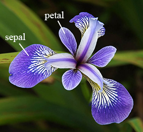
We can import and display the dataset description like this:
from sklearn.datasets import load_iris
iris = load_iris()
print(iris['DESCR'])
To get some idea of what the data looks like, let's look at scatter plots across each pair of features.
# code from
# http://stackoverflow.com/questions/21131707/multiple-data-in-scatter-matrix
from pandas.tools.plotting import scatter_matrix
import pandas as pd

iris_data = pd.DataFrame(data=iris['data'],columns=iris['feature_names'])
iris_data["target"] = iris['target']
color_wheel = {1: "#0392cf",
               2: "#7bc043",
               3: "#ee4035"}
colors = iris_data["target"].map(lambda x: color_wheel.get(x + 1))
ax = scatter_matrix(iris_data, color=colors, alpha=0.6, figsize=(15, 15), diagonal='hist')

We'll only select the first two flower classes for binary classification (~100 rows), and only use the first 2 features:
# Select first 2 flower classes (~100 rows)
# And first 2 features

sepal_len = iris['data'][:100,0]
sepal_wid = iris['data'][:100,1]
labels = iris['target'][:100]
We will also center the data. In this case, removing the mean means that we won't need a bias in our model and still get reasonable results. Our binary classification model will look like this:
\begin{align*} z &= w_1 x_1 + w_2 x_2 \\ y &= \sigma(z) \end{align*}
If $y >= 0.5$ then we will classify the flower as a Setosa.
sepal_len -= np.mean(sepal_len)
sepal_wid -= np.mean(sepal_wid)
Let's look at these two features. Note that in our case, the data set is linearly separable, meaning that it is possible to draw a line that separates the two classes.
plt.scatter(sepal_len,
            sepal_wid,
            c=labels,
            cmap=plt.cm.Paired)
plt.xlabel("sepal length")
plt.ylabel("sepal width")

Decision Boundaries
We can show that $y = \sigma(z) >= 0.5$ if and only if $z >= 0$. Meaning that the decision boundary $y = 0.5$ can be expressed as $w_1 x_1 + w_2 x_2 = 0$. The decision boundary is therefore a line through the origin in the data space!
The following function will help us plot a decision boundary $w_1 x_1 + w_2 x_2 = 0$. (You're not required to know how this code works.)
def plot_sep(w1, w2, color='green'):
    '''
    Plot decision boundary hypothesis
      w1 * sepal_len + w2 * sepal_wid = 0
    in input space, highlighting the hyperplane
    '''
    plt.scatter(sepal_len,
                sepal_wid,
                c=labels,
                cmap=plt.cm.Paired)
    plt.title("Separation in Input Space")
    plt.ylim([-1.5,1.5])
    plt.xlim([-1.5,2])
    plt.xlabel("sepal length")
    plt.ylabel("sepal width")
    if w2 != 0:
        m = -w1/w2
        t = 1 if w2 > 0 else -1
        plt.plot(
            [-1.5,2.0],
            [-1.5*m, 2.0*m],
            '-y',
            color=color)
        plt.fill_between(
            [-1.5, 2.0],
            [m*-1.5, m*2.0],
            [t*1.5, t*1.5],
            alpha=0.2,
            color=color)
    if w2 == 0: # decision boundary is vertical
        t = 1 if w1 > 0 else -1
        plt.plot([0, 0],
                 [-1.5, 2.0],
                 '-y',
                color=color)
        plt.fill_between(
            [0, 2.0*t],
            [-1.5, -2.0],
            [1.5, 2],
            alpha=0.2,
            color=color)
Let's look at a few example hypothesis to see how the choices of $w_1$ and $w_2$ influence the decision boundary:
# Example hypothesis
#   sepal_wid = 0

plot_sep(0, 1)

# Another example hypothesis:
#   -0.5*sepal_len + 1*sepal_wid >= 0

plot_sep(-0.5, 1)

# Another example hypothesis:
#   -1.5*sepal_len + 3*sepal_wid >= 0

plot_sep(-1.5, 3)
The decision boundary of the last two hypotheses look identical! Note that there is a difference
between the two models. For a flower with (mean-adjusted) sepal_length = 0 and sepal_width = -0.5,
the predictions for the two models are:
z1 = -0.5 * 0 + 1 * (-0.5)
y1 = 1 / (1 + np.exp(-z1))
print("Prediction for model 2: ", y1)

z2 = -1.5 * 0 + 3 * (-0.5)
y2 = 1 / (1 + np.exp(-z2))
print("Prediction for model 2: ", y2)
The second model will be more "certain" about its predictions.
Using sklearn
In project 1, you'll be writing code to use gradient descent to solve a linear classification problem. In practice, we use code that is already written and tested for us.
import sklearn.linear_model
model = sklearn.linear_model.LogisticRegression(fit_intercept=False)
model.fit(np.stack([sepal_len, sepal_wid], axis=1),
          labels)
Here are the coefficients that we get from sklearn:
model.coef_
plot_sep(3.02235857, -3.04217535)
