
State Estimation using Gaussian Process Regression
In today’s blogpost, we are turning to the problem of state estimation for continuum robots. While the modeling of continuum robots, which was covered by several previous blogposts, usually yields good agreement with respect to robotic prototypes, they are generally only accurate to a certain degree. Unlike models for rigid-link robots, which can be highly accurate, continuum robot models usually suffer from relatively high remaining errors due to unmodeled effects or other uncertainties arising from the elasticity of the material. While there might be merit in the effort of extending existing models to account for these effects, it also makes the models more complex and computationally expensive. This might make it challenging to apply such models in, for instance, real-time control settings.
Thus, state estimation approaches, which use additional sensor information to estimate the shape of continuum robots and can therefor account and compensate for such model inaccuracies, are promising. To this end, there is an open need for computationally efficient algorithms which can fuse models (which are known to be generally less accurate than for rigid robots) with appropriate measurements from sensors.
Througout the following, we want to give a brief overview on one particular method for the state estimation of continuum robots using Gaussian process regression, which we have recently published1 in the International Journal of Robotics Research in collaboration with Professor Tim Barfoot (ASRL, University of Toronto, Canada).
Simplified Cosserat Rod Model
For the prior of our state estimation algorithm, we use the well-known Cosserat rod model, which is commonly used in continuum robotics to model their kinematics and statics. Specifically, we are using a simplified version of this model, as shown in the figure below. The figure further highlights the similarities of the Cosserat rod model to the dynamics of a mobile robot, motivating the use of methods initially developed in that field of robotics.
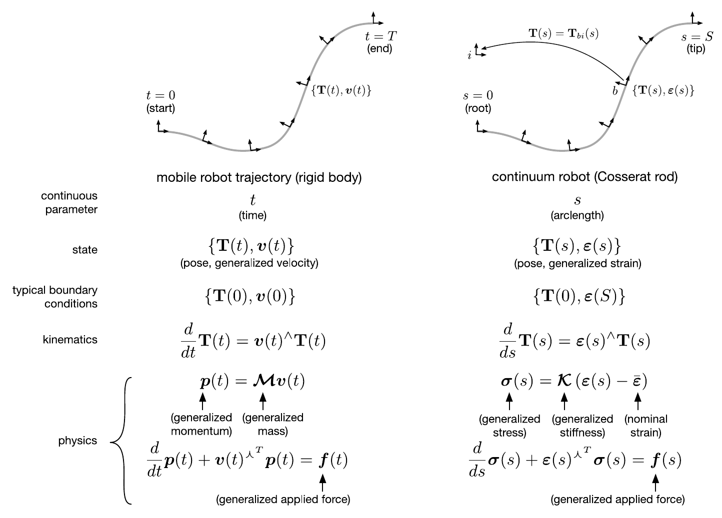 |
In fact, the method discussed in today’s blogpost has been initially developed for the continuous-time trajectory estimation of mobile robots and is repurposed to the continuous-shape estimation for continuum robots. In our case, the state that we want to estimate are the continuous shape, expressed as the pose \(\mathbf{T}(s)\), and strain \(\boldsymbol{\varepsilon}(s)\) along the arclength of a continuum robot, as opposed to the continuous pose and velocity of a mobile robot with respect to time. The equations above can be rearranged so that we obtain a system of ordinary differential equations that describe the derivatives of our desired state variables
\[\frac{d}{ds}\mathbf{T}(s) = \boldsymbol{\varepsilon}(s)^\wedge \mathbf{T}(s)\]and
\[\frac{d}{ds} \boldsymbol{\varepsilon}(s) = \boldsymbol{\mathcal{K}}^{-1}(\boldsymbol{f}(s)-\boldsymbol{\varepsilon}(s)^{\curlywedge^T} \boldsymbol{\sigma}(s))\]Gaussian Process Regression
In our work, we are using a batch state estimation framework in \(SE(3)\), which has first been proposed for the trajectory estimation of mobile robots by Anderson et al.2. In order to estimate the state of a continuum robot along its length, we want to derive a simple Gaussian process prior, including mean and covariance functions, in the following form: \(\mathbf{x}(s) \sim \mathcal{GP}( \check{\mathbf{x}}(s), \check{\mathbf{P}}(s,s^\prime))\)
The goal is to find expressions for the mean \(\check{\mathbf{x}}(s)\) and \(\check{\mathbf{P}}(s,s^\prime)\) covariance terms by corrupting the equations from the simplified Cosserat rod model with some process noise. We can achieve this, by replacing the derivative of the strain variables with respect to the arclength with a white-noise process. Our model now results in:
\[\frac{d}{ds}\mathbf{T}(s) = \boldsymbol{\varepsilon}(s)^\wedge \mathbf{T}(s)\] \[\frac{d}{ds} \boldsymbol{\varepsilon}(s) = \mathbf{w}(s)\] \[\mathbf{w}(s) \sim \mathcal{GP}( \mathbf{0}, \mathbf{Q}_c(s-s^\prime))\]where \(\mathbf{w}(s)\) is a white-noise Gaussian process with zero mean function and covariance function \(\mathbf{Q}_c(s-s^\prime)\). This leads to a rather general model, where no assumptions about both external or actuation forces are made. The advantage of this is, that we can apply the proposed state estimation approach to a wide variety of continuum robots that can be modeled using Cosserat rods.
One particular challenge now arises from the non-linearities in our differential equations for the pose variable, making it difficult to stochastically integrate them in order to obtain the expression for our Gaussian process. We can overcome this issue by discretizing our state into $K$ nodes along the robot arclength and then using multiple local Gaussian processes, defined using Lie algebra \(\mathfrak{se}(3)\), between those nodes. For this, we define local pose variables \(\boldsymbol{\xi}_k(s)\) in the corresponding Lie algebra \(\mathfrak{se}(3)\) that are connecting the poses between two discrete arclengths:
\[\mathbf{T}(s) = \underbrace{\exp\left( \boldsymbol{\xi}_k(s)^\wedge \right)}_{\in \, SE(3)} \mathbf{T}(s_k)\]This allows us to rewrite our differential equations with respect to the local variables as \(\frac{d}{ds} \begin{bmatrix} \boldsymbol{\xi}_k(s) \\ \boldsymbol{\psi}_k(s) \end{bmatrix} = \begin{bmatrix} \mathbf{0} & \mathbf{1} \\ \mathbf{0} & \mathbf{0} \end{bmatrix} \underbrace{\begin{bmatrix} \boldsymbol{\xi}_k(s) \\ \boldsymbol{\psi}_k(s) \end{bmatrix}}_{\boldsymbol{\gamma}_k(s)} + \begin{bmatrix} \mathbf{0} \\ \mathbf{1} \end{bmatrix} \mathbf{w}_k(s)\)
where \(\boldsymbol{\psi}_k(s)\) is the derivative of the local pose, \(\boldsymbol{\gamma}_k(s)\) is the Markovian state and \(\mathbf{w}_k(s)\) is again a zero-mean Gaussian process.
Integrating this equation in closed form yields us the following Gaussian process:
\[\boldsymbol{\gamma}_k(s) \sim \mathcal{GP} \bigl( \underbrace{\boldsymbol{\Phi}(s,s_k) \check{\boldsymbol{\gamma}}_k(s_k)}_{\rm mean~function}, \underbrace{\boldsymbol{\Phi}(s,s_k) \check{\mathbf{P}}(s_k) \boldsymbol{\Phi}(s,s_k)^T + \mathbf{Q}(s-s_k)}_{\rm covariance~function} \bigr)\]where \(\boldsymbol{\Phi}(s,s^\prime)\) is the transition function, \(\mathbf{Q}(s-s^\prime)\) is the covariance between two arclengths, and \(\check{\boldsymbol{\gamma}}_k(s_k)\) and \(\check{\mathbf{P}}(s_k)\) are the initial mean and covariance at the start of the local Gaussian process.
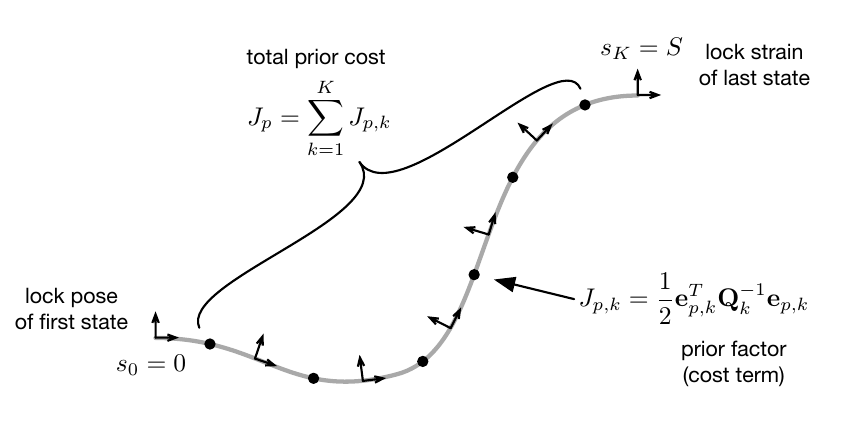
Given the expression for our Gaussian process, we can now construct an overall cost function, which depends on our state variables and whose minimum will be the posterior distribution of possible robot states.
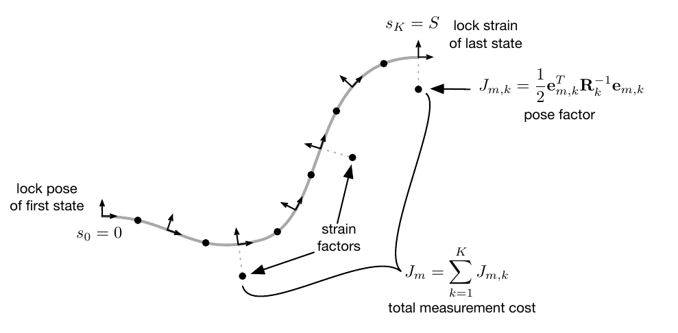
This cost function consists of two parts, one for the prior and one for measurements. For the prior, cost terms are added relating two neighbouring discrete states, penalizing deviations from our prior mean. For the measurements, terms are added, which relate sensor readings of the shape or strain at specific arclengths to the corresponding discrete states. Both cost terms are visualized as black dots in the factor graphs below.
 |
 |
For the sake of space, we won’t go into too much detail within this blogpost and refer interested readers to the derivations in our paper. The total cost to minimize can be obtained by summing up all individual cost terms. The resulting most-likely system state can be obtained by minimizing the resulting cost function with respect to the state variables:
\[\hat{\mathbf{x}} = \mbox{arg}\min_{\mathbf{x}} \sum_{k=1}^K J_{p,k} + \sum_{k=0}^K J_{m,k}\]This optimization can be performed by solving the linearized problem iteratively, for which the resulting system exhibits a highly sparse form that allows for efficient and fast computations. After the optimization, uncertainty information about the resulting estimate can be obtained using Laplace approximation. The details are again omitted here, but can be found in our paper.
Results and Conclusion
The figure below shows our state estimation approach in action to estimate the state of a two-segment tendon-driven continuum robot using two discrete pose measurements (located at the end of each segment).
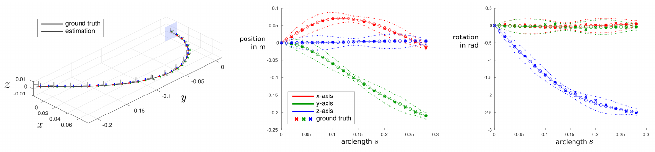
The resulting continuous shape estimate is shown with colored frames, while ground truth measurements are shown in gray. On the right, the \(x\)-, \(y\)- and \(z\)-components of the robot’s position and orientation with respect to its arclength are shown. The plots show the mean of the posterior distribution along with the 3$\sigma$ uncertainty envelopes and ground truth data (cross marks).
To summarize, the main benefits of our proposed approach are its universal applicability to most types of continuum robots, its fast computation times as well as the ability to interpolate the robot’s state and uncertainties at any arclength in a straightforward manner.
Further Reading: You can check out the theoretical and implementation details as well as our achieved results (both in simulation and experiments) in our open access publication1. For further reading on the state estimation in robotics, we point the reader to Tim Barfoot’s book on state estimation, which can serve as an excellent starting point and resource. Paper
References
-
Lilge S, Barfoot TD, Burgner-Kahrs J: Continuum robot state estimation using Gaussian process regression on SE(3). The International Journal of Robotics Research, 41(13-14):1099-1120, 2022. doi: 10.1177/02783649221128843 ↩ ↩2
-
Anderson S, Barfoot TD: Full STEAM Ahead: exactly sparse Gaussian process regression for batch continuous-time trajectory estimation on SE(3). IEEE/RSJ international conference on intelligent robots and systems (IROS), 2015. doi: 10.1109/IROS.2015.7353368 ↩