
Constant-Curvature Modeling of Concentric Tube Continuum Robots
Today, we are looking at how concentric tube continuum robots (CTCR) are modelled using the constant curvature kinematics framework. We derive the mapping for general CTCR composed of multiple tubes and then discuss the limitations.
Under the assumption that the robot’s shape is composed of constant curvature segments, it can be expressed as a concatenation of multiple circular arcs. Each circular arc corresponds to one segment \(i\) and each segment is described by its length \(\ell_{i}\), curvature \(\kappa_{i}\), and bending plane angle \(\phi_{i}\). To determine the robot dependent mapping for a CTCR, we need to identify the number \(m\) of segments present. As a segment is characterized by constant curvature, we have to locate transitions points along the robot where the curvature changes.
Robot Parameters
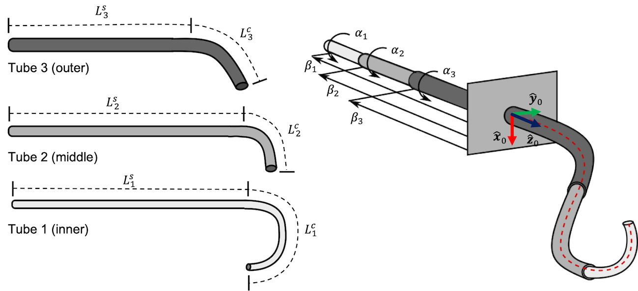
We identify a tube within the CTCR with index \(j \in \lbrack 1,N_{t}\rbrack\) where \(N_{t}\) is the number of tubes, \(j = 1\) is the innermost tube, and \(j = N_{t}\) is the outermost tube. Each tube is characterized by it length \(L_{j} = L_{j}^{s} + L_{j}^{c}\) where \(L_{j}^{s}\) is the length of the straight section and \(L_{j}^{c}\) is the length of the curved section (see Figure 5 left). We assume that the curved section has constant curvature \(\kappa_{j}^{*}\). The precurvature of a tube is defined in the xz-plane, where the z axis is tangential to the tube’s straight section pointing to the tip. Furthermore, each tube’s outer \(\text{OD}_{j}\) and inner \(\text{ID}_{j}\) diameter are specified. Lastly, the modulus of elasticity \(E_{j}\) (Young’s modulus) is determined by the tube’s material. Superelastic NiTi tubes typically come with elastic modulus of \(28 - 83\) GPa.
The CTCR joint space is given as \(\mathbf{q} = \lbrack\alpha_{1},\ldots,\alpha_{N_{t}},\beta_{1},\ldots,\beta_{N_{t}}\rbrack\) where \(\alpha_{j} \in \lbrack - \pi,\pi)\) is the rotation angle about the z-axis and \(\beta_{j} \in \lbrack - L_{j},0\rbrack\) is the translation along the z-axis of tube \(j\). If all \(\alpha_{j} = 0\), the centreline stays in the x-z-plane and curves toward the positive x axis. The translational joint variables are subject to the following constraints
\[\beta_{1} \leq \ldots \leq \beta_{N_{t}} \leq 0\]and
\[L_{N_{t}} + \beta_{N_{t}} \leq \ldots \leq L_{1} + \beta_{1}\]These arise from the telescoping nature of the tube assembly and the actuation principle, i.e., each tube can be retracted at maximum by its own length. Furthermore, we require the tubes to extend one another outside the actuation unit and to not be fully retracted within any more outer tube. In the robot’s zero position, all tubes are fully retracted and align with the front plate of the actuation unit. Below, we illustrate the joint space of a CTCR with \(N_{t} = 3\) and the base coordinate frame.
The robot dependent mapping is based on the principles of beam mechanics to solve the forward kinematic problem. We assume the tubes to deform only in bending and not in twisting, such that the resulting centerline curvature can be computed in closed-form based on a moment equilibrium by applying Bernoulli–Euler beam mechanics.
Resultant Curvature of Concentric Tubes
To describe the complete shape of a CTCR, we will first develop a model for the shape of a single segment composed of several fully overlapping concentric curved tubes. Let’s first consider the example depicted here.
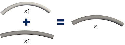
For a collection of two tubes with circular precurvatures \(\kappa_{1}^{*}\) and \(\kappa_{2}^{*}\), once inserted into each other, the resultant constant curvature \(\kappa\) is common to both tubes. Here, the tubes have not been axially rotated with respect to one another and their natural curvature planes are aligned. The bending moments \(M_{j}\) (in Nm) will be constant along the length of each tube and can be described by
\[M_{1} = (\kappa - \kappa_{1}^{*})EI_{1}\]and
\[M_{2} = (\kappa - \kappa_{2}^{*})EI_{2}\]where \(E\) is the Young’s modulus (in Pa), and \(I_{1}\) and \(I_{2}\) are
the second area moment (in \(m^{4}\)) of the symmetric cross section of
the respective tube. The second area moment \(I\) is a geometrical
property of the tube’s cross section area which reflects how its points
are distributed with regard to the central axis. As a
tube’s 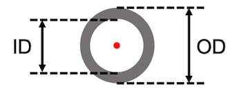 cross section is an annulus, the second
area moment can be determined from the inner and outer diameter as
cross section is an annulus, the second
area moment can be determined from the inner and outer diameter as
We can describe the resultant curvature of these two overlapping tubes by evaluating the moment equilibrium
\[M_{1} + M_{2} = 0\]and resolving for
\[\kappa = \frac{EI_{1}\kappa_{1}^{*} + EI_{2}\kappa_{2}^{*}}{EI_{1} + EI_{2}}\]This can be generalized to collections of \(N_{t}\) axially aligned tubes
\[\kappa = \frac{\sum_{j = 1}^{N_{t}}EI_{j}\kappa_{j}^{*}}{\sum_{j = 1}^{N_{t}}EI_{j}}\]Let’s now consider the example depicted here.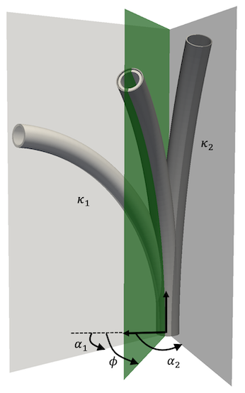 When precurved
tubes are rotated axially, their natural planes of curvature are no
longer aligned and the direction of the bending moments they apply
changes. The tubes exert a moment on one another about their respective
y-axes, which is caused by their initial precurvature about this
direction. The tubes are rotated by angles \(\alpha_{1}\) and
\(\alpha_{2}\), and the equilibrium plane angle is \(\phi\). As before, each
tube experiences a constant bending moment
\(M_{1} = (\kappa - \kappa_{1}^{*})EI_{1}\) and
\(M_{2} = (\kappa - \kappa_{2}^{*})EI_{2}\), but now these bending moments
have two component projections on the base frame x and y axes. The
equilibrium state \(M_{1} + M_{2} = 0\) yields
When precurved
tubes are rotated axially, their natural planes of curvature are no
longer aligned and the direction of the bending moments they apply
changes. The tubes exert a moment on one another about their respective
y-axes, which is caused by their initial precurvature about this
direction. The tubes are rotated by angles \(\alpha_{1}\) and
\(\alpha_{2}\), and the equilibrium plane angle is \(\phi\). As before, each
tube experiences a constant bending moment
\(M_{1} = (\kappa - \kappa_{1}^{*})EI_{1}\) and
\(M_{2} = (\kappa - \kappa_{2}^{*})EI_{2}\), but now these bending moments
have two component projections on the base frame x and y axes. The
equilibrium state \(M_{1} + M_{2} = 0\) yields
\(\begin{bmatrix} \kappa_{x} \\ \kappa_{y} \\ \end{bmatrix} = \frac{1}{EI_{1} + EI_{2}}\begin{pmatrix} EI_{1}\kappa_{1}^{*}\lbrack\begin{matrix} \cos\alpha_{1} \\ \sin\alpha_{1} \\ \end{matrix}\rbrack + EI_{2}\kappa_{2}^{*}\lbrack\begin{matrix} \cos\alpha_{2} \\ \sin\alpha_{2} \\ \end{matrix}\rbrack \\ \end{pmatrix}\).
For general number of concentric tubes, this can be generalized to
\[\begin{bmatrix} \kappa_{x} \\ \kappa_{y} \\ \end{bmatrix} = \frac{1}{\sum_{j = 1}^{N_{t}}EI_{j}}\overset{N_{t}}{\sum_{j = 1}}EI_{j}\kappa_{j}^{*}\begin{bmatrix} \cos\alpha_{j} \\ \sin\alpha_{j} \\ \end{bmatrix}(Eq. 1)\]Given the components of the resultant curvature, we can determine the bending plane angle \(\phi = \text{atan2}(\kappa_{y},\kappa_{x})\) and curvature \(\kappa = \sqrt{\kappa_{x}^{2} + \kappa_{y}^{2}}\). Note, that \(\phi\) is undefined for straight segments, i.e., for zero curvature as \(\text{atan}2(0,0) = \text{nan}\). In this special case, the rotation angle \(\alpha\) of the outermost present tube in the segment is used as \(\phi\).
Determining the Arc Parameters of a CTCR
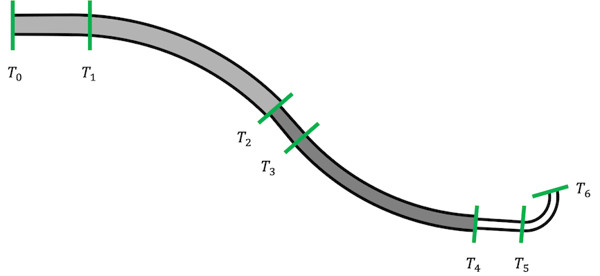
The first step in determining the robot dependent mapping of a CTCR is determining the number of segments \(m\) and their lengths \(\ell_{i}\) for \(i \in \lbrack 1,m\rbrack\). These are defined by transition point locations, where the component tubes either end or transition from their straight to curved section. The set \(T\) of transition points can be determined as algebraic functions of the tube geometry and the translational joint positions \(\beta_{j}\)
\[T = \text{sort}_{\text{asc}}\{ 0,\beta_{n} + L_{n}^{s},\beta_{n} + L_{n},\ldots\beta_{1} + L_{1}^{s},\beta_{1} + L_{1}\}\]From the resulting values of the set T, all duplicate elements are omitted, i.e., tube sections terminate at the same location, as well as all elements \(< 0\), i.e., the respective tube section is located within the actuation unit. While the maximum number of segments is \(2N_{t}\), the number of actual segments is dependent on the current joint values \(\mathbf{q}\) as some segments might be located within the actuation unit. Here, we show an example of a CTCR composed of three tubes and its transition points.
Using the transition points T, the length of the constant curvature segments of the CTCR can be determined as
\[\begin{matrix} \ell_{1} & = T_{1} - T_{0} \\ \ell_{2} & = T_{2} - T_{1} \\ \ldots & \\ \ell_{m} & = T_{m} - T_{m - 1} \\ \end{matrix}\]In a second step, we can determine \(\kappa_{x}\) and \(\kappa_{z}\) for each segment \(i \in \lbrack 1,m\rbrack\) enclosed by the transition points \(\lbrack T_{i - 1},T_{i}\rbrack\) using Equation (\(1\)), and then \(\kappa_{i}\) and \(\phi_{i}\). Note, that not all tubes are present in each segment, such that only the present ones with their respective parameters have to be considered (either zero curvature in straight tube sections or the respective precurvature in curved sections, alongside ID and OD, as well as \(E\)).
The constant curvature kinematics franmework assumes that \(\phi\) is expressed locally, i.e., w.r.t. the previous segment for the robot independent mapping. Consequently, after determining \(\phi_{i}\) expressed in the base frame for each segment using Equation (\(1\)), we will need to apply a final correction step
\(\phi_{i} = \phi_{i} - \phi_{i - 1}\).
Remarks
The model introduced today makes multiple simplifying assumptions, i.e., pure bending, no torsional deformation, no friction, no effect of gravitation and external forces. The assumption of infinite torsional rigidity in the tubes is only reasonable as long as the relative rotation angles between the tubes are small and the straight sections of each tube are short. Considering torsional deformation is particularly important in the straight transmission sections of the tubes that lie between the actuators and the first curved link, since these transmissions are long relative to the curved sections. In fact, despite the simple actuation of component tubes, the resulting motion of CTCR is characterized by a highly non-linear behaviour due to the elastic interactions between the tubes.
An advanced modelling approach is to leverage the elasticity theory, in particular the Cosserat theory of elastic rods. This involves writing rod equation for each tube, and then enforce concentricity by requiring all tubes to conform to the same curvature as a function of arc-length, leaving them free to rotate axially with respect to each other. This results in a system of differential equations with mixed boundary conditions. The boundary conditions at the base of the robot are the axial angles of the tubes, and the boundary conditions at the tip are internal moments that vanish because there is no material beyond the tip to support them. Note that after this mechanics problem is solved, to determine the axial tube angles, one must still integrate along the robot to determine the space curve of the robot itself. Experimental testing of the model has shown that with calibration, mean error in the prediction of tip position can be as low as 1% to 3% of overall robot length. With typical CTCR length of 200-300mm, this means that we can estimate the pose of the tip with an error of about 2-9 mm. This is the most accurate model existing for CTCR to date. As this 101 category of the OpenContinuumRobotics Blog is an introduction to continuum robotics, we do not cover advanced modelling approaches for CTCR (yet!).
Further Reading
Webster, R.J. & Jones, B.A., 2010. Design and Kinematic Modeling of
Constant Curvature Continuum Robots: A Review. The International Journal
of Robotics Research, 29(13), pp. 1661–1683.
https://doi.org/10.1177/0278364910368147
Section 3.2.3
Mahoney, A.W., Gilbert, H.B., Webster, R.J., 2018. A Review of Concentric Tube Robots: Modeling, Control, Design, Planning, and Sensing. The Encyclopedia of Medical Robotics, Chapter 7, pp. 181-202. https://doi.org/10.1142/9789813232266_0007