
Introduction to Modeling
Continuum robots are joint-less and composed of flexible, elastic, or soft materials. As such, they are continuously bending, eventually twisting and extending. In order to have a continuum robot do meaningful things, i.e. move along a predefined path, deploy into a cluttered environment, be teleoperated by a physician to help with brain surgery, we need to describe the relationship between joint space and task space. This kinematic mapping is essential for motion planning and control of any robot.
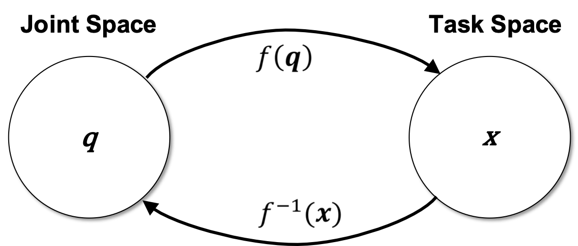
Mapping between Joint and Task Space
The term joint space may be confusing for continuum robots as we commonly think of revolute or prismatic joints. Those are not necessarily present in a continuum robot as actuation may be achieved by pulling on tendons or changing pressure in pneumatic components. Yet, we commonly refer to those actuator parameters as the robot’s joint space and we are interested in determining the relationship between joint space parameters and the resulting appearance of the robot in task space, i.e. its position and orientation at the tip or its shape.
Perhaps the most familiar kinematic modelling framework for roboticists is the discrete approach employed in conventional rigid-link manipulators: a series of rigid links connected by revolute, universal, or spherical joints is described using a series of homogeneous transformations, for example generated from Denavit Hartenberg (D-H) parameters or using the Product of Exponentials (PoE) formula. The underlying assumption, that the robot is composed of rigid-link and joints, does not hold for continuum robots. In fact, the body is continuously bending and the actuators/joints are not connected by rigid links. We could approximate the continuous structure of the robot’s body by a series of virtual joints and find a relationship between those virtual joints and the actual joint space. But the lack of distinct links in continuum robots makes the the D-H and PoE strategies, which define a finite number of coordinate frames (each fixed in one link), inappropriate for modelling. So rather than trying to fit a modelling approach to a continuum robot, it is more effective to utilize the structure and geometry of a continuum robot to come up with a more suitable kinematic framework.
We have seen several example continuum robots. From a mechanical standpoint, these continuum robots can be seen as slender structures, i.e. structures that are much longer in one direction than the other two directions. This slender structure is continuously bending and can be represented by a space curve.
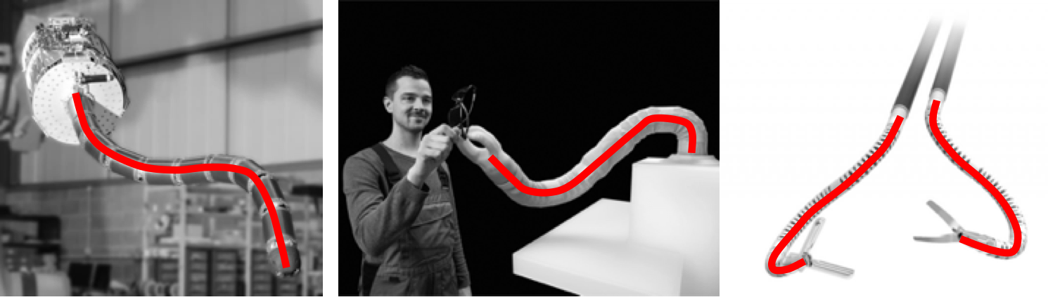 |
| (Images adapted, from left to right © OC Robotics Ltd, © FESTO, © Titan Medical Inc.) |
Therefore, we model continuum kinematics via a frame which evolves along a continuous backbone, parameterized by arc length \(s\). The local motion of the backbone at a point is modeled in terms of the local frame at s. This strategy allows computation of the forward kinematics and construction of continuum Jacobians, analogous to those for rigid-link systems. There exist multiple approaches on how this space curve can be determined based on the joint space parameters of a continuum robot. Those can be divided into mechanics-based frameworks and kinematic frameworks.
Mechanics-based Frameworks
Mechanics-based frameworks can either build on kinematics frameworks, such as lumped-parameter models, or build on classical elasticity theory for long slender objects such as rods and strings.
In lumped-parameter models, discrete mechanical elements such as point masses, springs, and dampers, are attached to the kinematic framework in order to approximate the mechanical behaviour of a continuous elastic and/or viscous medium. Governing equations can then be obtained from energy methods or Newton-Euler describing how forces and moments propagate from link to link.
In elasticity-based models, Cosserat rod theory and its special case Kirchhoff rod theory are commonly used to describe continuum robots. They resemble variable-curvature and typically describe a material-attached homogeneous reference frame comprising a position vector and a rotation matrix expressing the backbone pose as a function of arc length along the robot. The position vector and rotation both evolve along the arc length according to differential kinematic relationships. In addition, nonlinear ordinary differential equations are formulated for the equilibrium of internal forces and moments carried by the robot. The equilibrium equations are then coupled to the kinematic equations through some material constitutive law (stress–strain). The resulting set of equations can be solved subject to boundary conditions.
Today, we are focussing on the constant curvature kinematic framework, which is the most well-known and widely used kinematics framework for continuum robots. We will explore mechanics-based frameworks in future posts.
Constant Curvature Kinematic Framework
Notice that, independent of the underlying physical structure, a common property exhibited by the majority of continuum robots is that the resulting backbone can be approximated by a serially connected set of constant curvature sections. This arises due to the following: (1) all continuum robots, i.e. extrinsic and intrinsic actuated, create a series of connected sections; and (2) internal potential energy in each section is uniformly distributed (each section is initially straight, or bent at a fixed configuration); and thus, within each section, internal forces act to drive the unactuated (passive) degrees of freedom to equalize in value along the section. This produces internal section bending of constant curvature at any given point in time. Therefore, in practice, achievable continuum backbone shapes are (fairly close approximations to) sequentially connected segments of circles or helices in three dimensions, with the tangents to successive section end points aligned and the arc lengths of the segments corresponding to robot section lengths.
Constant curvature kinematic frameworks represent the continuum robot’s configuration space as a finite number of mutually tangent curved segments each having a constant curvature along its length. Note that constant here refers to invariance with respect to arc length, not time. In this framework, the curvature, length, and angle of the curve’s bending plane - known as the arc parameters - of each segment form a set of configuration coordinates that completely describes the shape of the robot. The position and orientation at any point on the robot, can be written as a function of the arc parameters and the arc length along the backbone to that point. Similar to D-H parameters, an arc parameter could be a constant or vary with actuation, depending on the robot design. Usually, a single constant-curvature segment is employed for each actuatable segment of the robot.
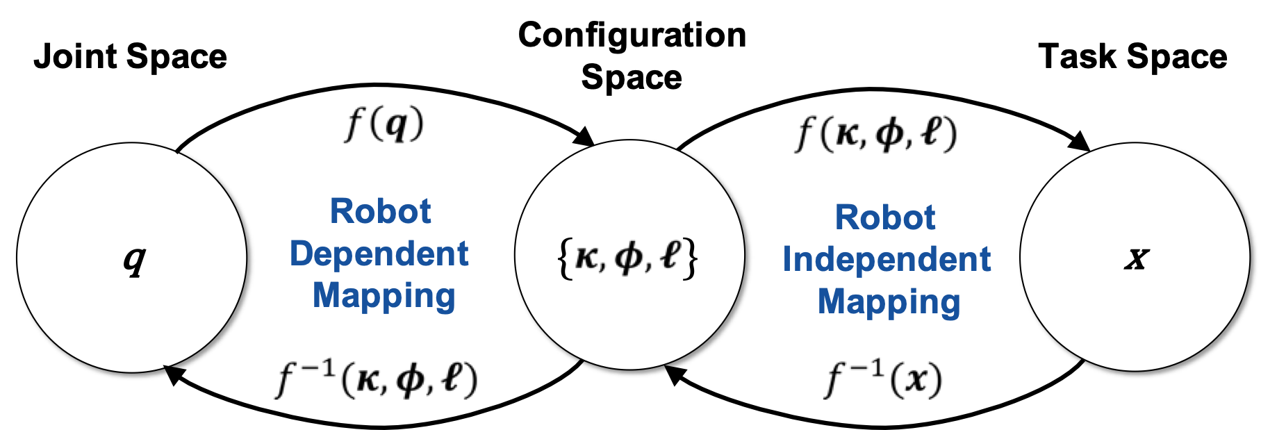
The forward kinematics of a continuum robot refers to the calculation of the position and orientation of its tip from its joint coordinates. The arc parameters are determined as an intermediate step in this calculation, which is the robot dependent mapping from joint space to configuration space as it depends on the robot’s mechanical structure and actuation principle employed. Using these configuration space parameters, the robot independent mapping determines the task space parameters.
Consequently, the inverse kinematics is also decomposed into two mappings. The robot independent inverse mapping from task space to geometrical parameters relates the desired position or pose of the robot’s tip to arc parameters. The robot dependent inverse mappings then determines the respective joint space parameters in order to achieve the arc parameters for each segment. In general, the inverse kinematics of continuum robots is challenging to derive as the number of solutions is not definite and a closed-form solution does not necessarily exist.
Remarks
Constant curvature is often referred to as the constant curvature assumption, but care must be taken when using this phrase because it may not always accurately describe the methodology used in developing a constant-curvature model. One can indeed make an a priori assumption of piecewise constant curvature and subsequently formulate mechanics relationships and robot models under that assumption. However, a constant-curvature robot shape also arises as a natural result from mechanical principles when certain robot designs and assumptions are considered within a more general variable-curvature framework.
The accuracy of constant curvature kinematic frameworks is contingent on the actual continuum robot and how well it suits the modelling assumption. The inevitable tradeoffs between model complexity, computational expense, and accuracy are the primary principles that should be considered when modelling continuum robots. We look into the accuracy and limitations of the constant curvature kinematic framework for different continuum robot types in our next blog posts.
Further Reading: Curious about modeling and can’t wait for the next 101 blog post going into more detail? Webster & Jones1 published a beginner-friendly review on modeling continuum robots using the constant curvature framework.
References
-
Webster, R.J. & Jones, B.A., 2010. Design and Kinematic Modeling of Constant Curvature Continuum Robots: A Review. The International Journal of Robotics Research, 29(13), pp. 1661–1683.doi: 10.1177/0278364910368147 ↩