The Two Cultures, and a Predictive Workflow
Breiman’s two cultures
Leo Breiman — a Berkeley statistician — wrote a famous 2001 essay, “Statistical Modeling: The Two Cultures,” telling the story of his own move from one half of this course to the other. He identifies two ways to analyze data:
- The data-modeling culture. Assume a model of how the data was generated — a mechanism, a causal structure — fit it, and draw conclusions about the world from it. This is the first half of the course: probability models, maximum likelihood, Bayesian inference, hypothesis testing, causal inference.
- The algorithmic (predictive) culture. Admit you don’t know the true data-generating mechanism, and don’t try to. Just take the inputs and predict the outputs as accurately as possible. This is the second half: predictive modeling, cross-validation, trees and forests, neural networks.
The trade is real. The predictive culture often predicts better — especially on high-dimensional data like images — but it buys accuracy at the price of understanding: a model tuned only to predict licenses no claims about how the world works. (Your instructor leans culture-1 philosophically: prediction is useful but “can only get you so far” — you can say what you’d have predicted, not why.) Sometimes you can peek inside a complex model (which hidden unit detects what — see the neural networks notes), but those interpretations are shaky.
The course so far, in one frame
Inference (culture 1). The core question is often “is \(X\) merely associated with \(Y\)?” You can answer it:
- by hand — simulate fake data under the null and see whether the real data is consistent with it (hypothesis testing);
- by looking up a test — usually faster, and usually applied slightly incorrectly, because the standard test’s model is rarely exactly right;
- with a custom generative model — write your own data-generating process, simulate, and test;
- Bayesianly — get actual probabilities you can believe, at the cost of needing a prior (Bayesian inference).
None of that is causal inference. There is a causal structure to real data, but you usually don’t know it; only in well-studied areas do you have the pieces (how flossing affects inflammation, how inflammation affects heart disease…) to attempt it (causal inference).
Prediction (culture 2). Many models — linear/logistic regression, trees, neural networks. Complex models often (not always) predict better, especially in high dimensions; interpreting them is possible but limited.
The rest of these notes is a culture-2 worked example: predicting a tournament.
Worked example: predicting the World Cup
The goal: build a full bracket — a predicted winner for each game, and overall finishing odds. This is pure predictive culture: we make no claim about why teams win, only about who probably will.
Where do the input probabilities come from?
Not FIFA rankings — they update slowly and ignore that some teams landed in harder groups. A better source is a prediction market.
Prediction markets. A site where people bet on outcomes. If a “yes” share for Spain wins the World Cup trades at 16.6¢ — pay 16.6¢ now, receive $1 if Spain wins — the market is implicitly pricing Spain’s chance at about 17%. The site acts as a broker: as demand for “yes” rises, its price rises. For heavily-traded events these implied probabilities are usually more reliable than slow official rankings — when a goal is scored mid-game, prices adjust in seconds. (This is a lens on probability, not a betting recommendation.)
Getting the data with an agent
You don’t need a scraper. A quick, reliable workflow:
# 1. Select-all / copy the market's probabilities from the web page,
#    paste into polymarket_raw.txt.
# 2. Ask the coding agent:
"Turn polymarket_raw.txt into a tidy CSV: columns team, win_prob."
# 3. And, in parallel:
"Scrape the latest FIFA men's ranking into fifa.csv."
Copy-paste → “make me a CSV” is often faster and more robust than scraping ad-heavy sites like Polymarket — and you can verify the small CSV by eye. FIFA serves here only as a tiebreaker (the market rates all the no-hope teams identically).
From ratings to match outcomes
Give each team a strength, and turn the difference in strength into a match probability with the logistic function from logistic regression: a bigger edge → a higher win probability, squashed into \([0,1]\).
# Win probability for A vs B as a logistic function of the rating gap.
p_win <- function(rating_a, rating_b, scale = 0.9) {
  plogis(scale * (rating_a - rating_b))
}
p_win(2.0, 1.0)   # a one-point-stronger team
## [1] 0.7109495p_win(1.0, 1.0) # evenly matched -> 0.5## [1] 0.5Group games can end in draws, so we carve the same logistic score into loss / draw / win bands — a modeling choice you then sanity-check by simulating a few games and seeing whether the mix looks plausible (not all draws, not the same team always winning):
outcome_probs <- function(rating_a, rating_b, scale = 0.9) {
  s <- plogis(scale * (rating_a - rating_b))   # in (0,1)
  # Map the score to (loss, draw, win). Draws most likely for even games.
  draw <- 0.30 * (1 - abs(2 * s - 1))          # peaks at s = 0.5
  win  <- (1 - draw) * s
  loss <- (1 - draw) * (1 - s)
  c(loss = loss, draw = draw, win = win)
}
round(outcome_probs(2.0, 1.0), 2)   # stronger team: win most likely
## loss draw win
## 0.24 0.17 0.59round(outcome_probs(1.0, 1.0), 2) # even: draw inflated, win = loss## loss draw win
## 0.35 0.30 0.35Why simulate rather than just rank?
Because the bracket structure matters: a strong team in a brutal group can be knocked out early, and raw rankings can’t see that. So we simulate the whole tournament many times and count how often each team advances — a Monte-Carlo estimate of finishing odds.
set.seed(1626)

# Illustrative strengths (NOT real market numbers) for eight teams.
teams <- c(Spain = 2.4, France = 2.3, Brazil = 2.2, Argentina = 2.1,
           England = 1.8, Portugal = 1.7, Netherlands = 1.5, Canada = 1.0)

# One single-elimination match: stronger team wins with prob p_win
# (knockouts have no draws — a shootout resolves them).
play <- function(a, b) if (runif(1) < p_win(teams[a], teams[b])) a else b

simulate_bracket <- function() {
  round <- names(teams)                 # 8-team bracket, seeded 1..8
  while (length(round) > 1) {
    winners <- character(0)
    for (i in seq(1, length(round), by = 2))
      winners <- c(winners, play(round[i], round[i + 1]))
    round <- winners
  }
  round                                 # the champion
}

champions <- replicate(2000, simulate_bracket())
title_odds <- sort(table(champions) / length(champions), decreasing = TRUE)
round(title_odds, 3)
## champions
## Spain France Brazil Argentina England Portugal
## 0.195 0.168 0.156 0.133 0.124 0.106
## Netherlands Canada
## 0.088 0.030odds_df <- data.frame(team = names(title_odds), prob = as.numeric(title_odds))
ggplot(odds_df, aes(reorder(team, prob), prob)) +
geom_col(fill = "steelblue") + coord_flip() +
labs(x = NULL, y = "simulated title probability",
title = "World Cup title odds from 2000 simulated brackets")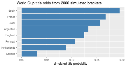
Notice how the small per-game edges compound: the favourite is barely ahead of the second seed in any single match, yet ends up with a clearly larger title probability, and it sits well above the even 1-in-8 (0.125) a coin-flip bracket would give. That amplification — the “rich get richer” — is exactly what raw rankings miss and simulation captures. If you fed the market’s own numbers in, you could even re-tune scale until the simulation is self-consistent with the market.
Trust, but audit
The agent will happily run all this, and it makes mistakes — here it repeatedly grabbed data it already had, and once computed standings for the groups instead of the tournament. If you were betting real money you’d audit the generated code; for a low-stakes office pool, less so. The honest takeaway: the optimal bracket is “the market’s probabilities, plus your own hot takes” — and the point of the exercise is that assembling this whole predictive pipeline, agent and all, is now something you can do in an afternoon.
Summary
- Breiman’s two cultures: model the data-generating mechanism and infer about the world (culture 1) vs. predict the output as well as possible with no such claims (culture 2). This course does both halves, in that order.
- Culture 2 buys predictive accuracy at the cost of understanding; culture 1 buys understanding at the cost (often) of predictive power.
- Prediction markets turn prices into calibrated-ish probabilities — a good predictive input.
- A predictive workflow in practice: pull probabilities, convert rating gaps to outcome probabilities with the logistic function, simulate the whole bracket (Monte Carlo) to respect its structure, and audit the agent’s code.
References
- Breiman (2001), “Statistical Modeling: The Two Cultures,” Statistical Science.
- Ties together hypothesis testing (simulation), logistic regression (the outcome model), causal inference, and neural networks (culture-2 models).