Wrangling Data with the Pipe and `tidyverse` / `dplyr`

Function composition

Before we get to tidyverse, we just want to think about function composition for a moment. This is the kind of thing that everyone knows already, but we are thinking about it just for the sake of getting into the rhythm.

If f(x) = x^2 and g(y) = y + 1, then in math:

\[f(g(5)) = (5+1)^2 = 36\]

In R:

f <- function(x){ x ** 2 }
g <- function(y){ y + 1 }
f(g(5))

## [1] 36

The pipe operator

In R there is a shorthand for function composition called the pipe operator %>%. The expression 5 %>% g() %>% f() means “take 5, plug it into g, then plug the result into f”:

5 |> g() |> f()

## [1] 36

One downside is that the pipe is annoying to type. In RStudio (with the R extension installed), Ctrl+Shift+M produces the pipe. The arrow <- is Alt+-.

The reason this is useful is that it is a good way to think about data frames.

square <- function(y){ y ** 2 }
5 |> g() |> square()

## [1] 36

`tidyverse` and `dplyr` verbs

Let’s load tidyverse and the babynames data set:

library(dplyr)
library(ggplot2)
library(tidyr)
library(babynames)

`filter` for rows

filter selects rows. The following are all equivalent — different ways of selecting rows for which the year is 1880 and the sex is "F":

filter(babynames, year == 1880, sex == "F")
idx <- (babynames$year == 1880) & (babynames$sex == "F")
babynames[idx, ]
babynames |> filter(year == 1880 & sex == "F")
babynames |> filter(year == 1880, sex == "F")

The pipe form reads nicest. Technically it is just calling the function filter; it is just more convenient to write this way. filter can take several conditions joined with commas (equivalent to &).

`select` for columns

select produces a new data frame with the specified columns (in the order you specify):

babynames |> select(year, name) |> head()

## # A tibble: 6 × 2
##    year name     
##   <dbl> <chr>    
## 1  1880 Mary     
## 2  1880 Anna     
## 3  1880 Emma     
## 4  1880 Elizabeth
## 5  1880 Minnie   
## 6  1880 Margaret

It is kind of “filter for columns” — get a new data frame with just those specific columns.

`arrange` for sorting

arrange produces a data frame sorted by the column(s) you specify. babynames happens to be sorted by year already:

babynames |> arrange(n) |> head()

## # A tibble: 6 × 5
##    year sex   name          n      prop
##   <dbl> <chr> <chr>     <int>     <dbl>
## 1  1880 F     Adelle        5 0.0000512
## 2  1880 F     Adina         5 0.0000512
## 3  1880 F     Adrienne      5 0.0000512
## 4  1880 F     Albertine     5 0.0000512
## 5  1880 F     Alys          5 0.0000512
## 6  1880 F     Ana           5 0.0000512

This is sorted in increasing order, so it shows the rarest entries. To sort in descending order, which is the more interesting thing because you want the most common ones:

babynames |> arrange(desc(n)) |> head()

## # A tibble: 6 × 5
##    year sex   name        n   prop
##   <dbl> <chr> <chr>   <int>  <dbl>
## 1  1947 F     Linda   99686 0.0548
## 2  1948 F     Linda   96209 0.0552
## 3  1947 M     James   94756 0.0510
## 4  1957 M     Michael 92695 0.0424
## 5  1947 M     Robert  91642 0.0493
## 6  1949 F     Linda   91016 0.0518

You can combine with filter:

babynames |> filter(year == 2000) |> arrange(desc(n)) |> head(10)

## # A tibble: 10 × 5
##     year sex   name            n   prop
##    <dbl> <chr> <chr>       <int>  <dbl>
##  1  2000 M     Jacob       34471 0.0165
##  2  2000 M     Michael     32035 0.0153
##  3  2000 M     Matthew     28572 0.0137
##  4  2000 M     Joshua      27538 0.0132
##  5  2000 F     Emily       25953 0.0130
##  6  2000 M     Christopher 24931 0.0119
##  7  2000 M     Nicholas    24652 0.0118
##  8  2000 M     Andrew      23639 0.0113
##  9  2000 F     Hannah      23080 0.0116
## 10  2000 M     Joseph      22825 0.0109

If you want the top 10 female names in 2000:

babynames |> filter(year == 2000, sex == "F") |> arrange(desc(n)) |> head(10)

## # A tibble: 10 × 5
##     year sex   name          n    prop
##    <dbl> <chr> <chr>     <int>   <dbl>
##  1  2000 F     Emily     25953 0.0130 
##  2  2000 F     Hannah    23080 0.0116 
##  3  2000 F     Madison   19967 0.0100 
##  4  2000 F     Ashley    17997 0.00902
##  5  2000 F     Sarah     17697 0.00887
##  6  2000 F     Alexis    17629 0.00884
##  7  2000 F     Samantha  17266 0.00866
##  8  2000 F     Jessica   15709 0.00787
##  9  2000 F     Elizabeth 15094 0.00757
## 10  2000 F     Taylor    15078 0.00756

You can arrange by multiple columns: arrange(year, name) sorts by year, then within each year by name.

`rename`

babynames |> rename(number = n) |> head()

## # A tibble: 6 × 5
##    year sex   name      number   prop
##   <dbl> <chr> <chr>      <int>  <dbl>
## 1  1880 F     Mary        7065 0.0724
## 2  1880 F     Anna        2604 0.0267
## 3  1880 F     Emma        2003 0.0205
## 4  1880 F     Elizabeth   1939 0.0199
## 5  1880 F     Minnie      1746 0.0179
## 6  1880 F     Margaret    1578 0.0162

This is sometimes useful because n is also a function (we will see that in a second).

`select` with renaming

You can rename as you select. This gives you a data frame with year, sex, and number instead of n:

babynames |> select(year, sex, number = n) |> head()

## # A tibble: 6 × 3
##    year sex   number
##   <dbl> <chr>  <int>
## 1  1880 F       7065
## 2  1880 F       2604
## 3  1880 F       2003
## 4  1880 F       1939
## 5  1880 F       1746
## 6  1880 F       1578

This is equivalent to:

babynames |> rename(number = n) |> select(year, sex, number)

`mutate` for adding a column

mutate adds one more column; the column can be whatever you want.

The way babynames works, you have n (count) and prop (proportion). So 7% of female babies, say, are named Mary. If you want to reconstruct the population, you can divide n by prop:

babynames |> mutate(total_by_year = round(n / prop)) |> head()

## # A tibble: 6 × 6
##    year sex   name          n   prop total_by_year
##   <dbl> <chr> <chr>     <int>  <dbl>         <dbl>
## 1  1880 F     Mary       7065 0.0724         97605
## 2  1880 F     Anna       2604 0.0267         97605
## 3  1880 F     Emma       2003 0.0205         97605
## 4  1880 F     Elizabeth  1939 0.0199         97605
## 5  1880 F     Minnie     1746 0.0179         97605
## 6  1880 F     Margaret   1578 0.0162         97605

In the first 10 rows, total_by_year is all the same — that’s because they are all 1880, and the number of Marys divided by the proportion of Marys equals the number of Janes divided by the proportion of Janes, etc.

`summarize`

summarize creates a new data frame where there is a new column (you can have several), and the column is a function of the columns of the original data frame:

babynames |> summarize(mean_n = mean(n))

## # A tibble: 1 × 1
##   mean_n
##    <dbl>
## 1   181.

So this took the column n and computed the mean of it. mean is just a function like any other; you plug in a vector and get the mean.

By itself this is not that useful, but it becomes useful when you can group:

babynames |> group_by(sex) |> summarize(mean_n = mean(n))

## # A tibble: 2 × 2
##   sex   mean_n
##   <chr>  <dbl>
## 1 F       151.
## 2 M       223.

This separates the data frame out by the different sexes and computes the mean of n for each. So this is the mean number of babies born per name, by sex. As it happens, in the US data set, there are more babies per name that are male than female — there is basically more diversity in female names. It’s approximately the same number of male and female babies; it’s just that there are fewer male names. So more babies per name as it turns out.

`distinct`

distinct is kind of similar to unique except it operates by row. It says: get me all the rows that are different.

Let’s reconstruct the per-year total population:

b_tot <- babynames |> mutate(total = round(n / prop))
b_tot |> head()

## # A tibble: 6 × 6
##    year sex   name          n   prop total
##   <dbl> <chr> <chr>     <int>  <dbl> <dbl>
## 1  1880 F     Mary       7065 0.0724 97605
## 2  1880 F     Anna       2604 0.0267 97605
## 3  1880 F     Emma       2003 0.0205 97605
## 4  1880 F     Elizabeth  1939 0.0199 97605
## 5  1880 F     Minnie     1746 0.0179 97605
## 6  1880 F     Margaret   1578 0.0162 97605

All the rows here are unique because the (year, name) combinations are unique. But if we drop the name, n, and prop columns, lots of rows become the same — because it’s just (year, sex, total).

b_tot |> select(year, sex, total) |> distinct() |> head()

## # A tibble: 6 × 3
##    year sex   total
##   <dbl> <chr> <dbl>
## 1  1880 F     97605
## 2  1880 F     97604
## 3  1880 F     97606
## 4  1880 F     97603
## 5  1880 F     97607
## 6  1880 F     97602

So distinct is like unique but for rows. (The numbers are not quite equal across names within a year, just because of rounding.)

You can also do distinct(year) to get all the different years:

babynames |> distinct(year) |> head()

## # A tibble: 6 × 1
##    year
##   <dbl>
## 1  1880
## 2  1881
## 3  1882
## 4  1883
## 5  1884
## 6  1885

distinct(year, name) gets all distinct (year, name) combinations.

`summarize` with multiple columns

babynames |> summarize(mean_n = mean(n), median_n = median(n))

## # A tibble: 1 × 2
##   mean_n median_n
##    <dbl>    <int>
## 1   181.       12

group_by followed by mutate lets you do per-group proportions:

babynames |> group_by(year, sex) |>
  summarize(total = sum(n)) |>
  head()

## # A tibble: 6 × 3
## # Groups:   year [3]
##    year sex    total
##   <dbl> <chr>  <int>
## 1  1880 F      90993
## 2  1880 M     110491
## 3  1881 F      91953
## 4  1881 M     100743
## 5  1882 F     107847
## 6  1882 M     113686

`n_distinct` and the `n` function

n_distinct(...) is the number of distinct rows in a data frame (recall that for vectors we could use length(unique(v))).

Here we count the number of distinct names for each sex × year:

babynames |> group_by(sex, year) |>
  summarize(distinct_names = n_distinct(name)) |>
  head()

## # A tibble: 6 × 3
## # Groups:   sex [1]
##   sex    year distinct_names
##   <chr> <dbl>          <int>
## 1 F      1880            942
## 2 F      1881            938
## 3 F      1882           1028
## 4 F      1883           1054
## 5 F      1884           1172
## 6 F      1885           1197

The n() function can be used inside summarize, mutate, and filter. Its job is to count the number of rows in each group:

babynames |> rename(num = n) |> summarize(total_entries = n())

## # A tibble: 1 × 1
##   total_entries
##           <int>
## 1       1924665

(Not quite the same as all the name-year combinations: babynames %>% summarize(name_year_count = n_distinct(year, name)).)

`which.max`

which.max(c(10, 20, 3, 10)) returns the location (index) of the maximum.

which.max(c(10, 20, 3, 10))

## [1] 2

What is the most popular name every year, by sex?

babynames |> group_by(year, sex) |>
  summarize(most_popular_name = name[which.max(n)]) |>
  head()

## # A tibble: 6 × 3
## # Groups:   year [3]
##    year sex   most_popular_name
##   <dbl> <chr> <chr>            
## 1  1880 F     Mary             
## 2  1880 M     John             
## 3  1881 F     Mary             
## 4  1881 M     John             
## 5  1882 F     Mary             
## 6  1882 M     John

It is John in 1880 for M; over the years it changes. With group_by, the table gets split per year × sex, and we ask name[which.max(n)] for each group.

Worked example: distinct names per capita

We compute the number of distinct names per capita, every year, for sex == "F":

name_per_cap <- babynames |> filter(sex == "F") |>
  group_by(year) |>
  summarize(distinct_names = n_distinct(name),
            total_by_year = sum(n)) |>
  mutate(distinct_per_capita = distinct_names / total_by_year) |>
  select(year, distinct_per_capita)

plot(name_per_cap$year, name_per_cap$distinct_per_capita)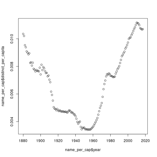

Let’s read this together. group_by(year) means one row per year. filter(sex == "F") means we are just within F rows. We compute two columns: distinct_names is the number of distinct names within the (year) data frame, and total_by_year is the sum of n. Now we are inside this guy: we want distinct_per_capita, which is distinct_names / total_by_year. This is a mutate because we are adding another column, not grouping. Then we just keep year and distinct_per_capita.

There were fewer names in 1950 — everyone had the same name. Things got more diverse recently.

To do it for both M and F at the same time, just add sex to the group:

name_per_cap_2 <- babynames |>
  group_by(year, sex) |>
  summarize(distinct_names = n_distinct(name),
            total_by_year = sum(n)) |>
  mutate(distinct_per_capita = distinct_names / total_by_year) |>
  select(year, sex, distinct_per_capita)
head(name_per_cap_2)

## # A tibble: 6 × 3
## # Groups:   year [3]
##    year sex   distinct_per_capita
##   <dbl> <chr>               <dbl>
## 1  1880 F                 0.0104 
## 2  1880 M                 0.00958
## 3  1881 F                 0.0102 
## 4  1881 M                 0.00990
## 5  1882 F                 0.00953
## 6  1882 M                 0.00967

Should we compute names per capita or total names?

There are arguments either way.

Why compute the total number of names? We are interested in how diverse the names are in the US. In some sense the population is irrelevant — if there are 50,000 names available to choose from, that’s interesting regardless of the fact that the population is very large. It is a question of how people are naming, not how many people there are.
Why compute the number of names per capita? If there are only 1,000 babies born, there cannot be more than 1,000 unique names. If there are 1,000 newborns and each of them has a unique name, that indicates that the names are very diverse.
Maybe we should do neither? Perhaps a compromise would be to compute the number of unique names per cultural or linguistic group — but that is difficult to define. If the population is larger you would expect more cultural groups just because a smaller population cannot support many distinct cultural groups; if you want an overall trend you’d actually need to separate out by cultural groups, average per cultural group, then aggregate.

`gapminder` mini-tour

The gapminder data set is a dataset of countries with life expectancy, population, GDP per capita for different years:

library(gapminder)
head(gapminder)

## # A tibble: 6 × 6
##   country     continent  year lifeExp      pop gdpPercap
##   <fct>       <fct>     <int>   <dbl>    <int>     <dbl>
## 1 Afghanistan Asia       1952    28.8  8425333      779.
## 2 Afghanistan Asia       1957    30.3  9240934      821.
## 3 Afghanistan Asia       1962    32.0 10267083      853.
## 4 Afghanistan Asia       1967    34.0 11537966      836.
## 5 Afghanistan Asia       1972    36.1 13079460      740.
## 6 Afghanistan Asia       1977    38.4 14880372      786.

How many countries on a given continent

One way: filter, get the countries, unique them, take the length.

asia <- gapminder |> filter(continent == "Asia")
length(unique(asia$country))

## [1] 33

A more idiomatic way:

gapminder |> filter(continent == "Asia") |>
  select(country) |>
  distinct() |>
  count()

## # A tibble: 1 × 1
##       n
##   <int>
## 1    33

Country with largest life expectancy on a continent between years `y1` and `y2`

top_country <- function(continent_name, y1, y2){
  g1 <- gapminder |>
    filter(continent == continent_name,
           year >= y1,
           year <= y2)
  g1$country[g1$lifeExp == max(g1$lifeExp)]
}
top_country("Asia", 1970, 1980)

## [1] Japan
## 142 Levels: Afghanistan Albania Algeria Angola Argentina Australia ... Zimbabwe

Note the >= and <=: gapminder samples years every five years (1952, 1957, …, 2007), so strict inequalities year > 1970 and year < 1980 would catch no rows at all (nothing in the data is strictly between 1970 and 1980). It’s a common gotcha with this dataset.

World population in a given year

We want the sum of all populations, by year. With group_by(year) and summarize(sum(pop)):

world_pop <- gapminder |> group_by(year) |> summarize(total = sum(pop))
world_pop |> filter(year == 1982)

## # A tibble: 1 × 2
##    year      total
##   <int>      <dbl>
## 1  1982 4289436840

world_pop |> filter(year == 2007)

## # A tibble: 1 × 2
##    year      total
##   <int>      <dbl>
## 1  2007 6251013179

4.3 billion in 1982 and 6.2 billion in 2007 — that sounds about right.

`sapply` and vector-safe functions

If what you have is a function that is just x^2, you can apply it to a vector directly — it just works:

square <- function(x){ x ** 2 }
vec <- c(1, 2, 4, 5)
square(vec)

## [1]  1  4 16 25

This only works for algebraic expressions. If you have something like:

special.square <- function(x){
  if(x == 42){
    42
  } else {
    x ** 2
  }
}

then special.square(vec) produces an error, because if(c(F, F, F, F)) does not make sense — there has to be one logical value inside the if.

If what you want is to apply special.square to every element of vec, use sapply:

vec <- c(1, 2, 42, 5)
sapply(X = vec, FUN = special.square)

## [1]  1  4 42 25

sapply applies the function specified by FUN to every element of the vector after X. (FUN is short for “function”, not “fun”; though it kind of is fun.)

You can also call without named arguments — sapply(vec, special.square) — but using named arguments makes things clear.

Nothing conceptually complicated here. It is just for-loop logic re-expressed as a function call. R does have for loops as well; it is just that in the style we are working in, you can also do sapply. R also happens to run sapply faster than the equivalent for loop.

`sapply` with extra arguments

Suppose we want to compute elem - 2 for every element elem in a vector using the function minus:

minus <- function(a, b){ a - b }
vec <- c(5, -6, 7, -8)
sapply(X = vec, FUN = minus, b = 2)

## [1]   3  -8   5 -10

We can specify that the 2 is sent into b. Note that X = vec is special: that will be the first argument given to minus, i.e. every element of X = vec will be sent to a.

Function composition

The pipe operator

tidyverse and dplyr verbs

filter for rows

select for columns

arrange for sorting

rename

select with renaming

mutate for adding a column

summarize

distinct

summarize with multiple columns

n_distinct and the n function

which.max