Decision Trees (and k-Nearest-Neighbours)
Alongside neural networks, the other workhorse for prediction — especially on tabular data — is the decision tree, and its ensemble cousin the random forest. We’ll motivate them by comparing how different classifiers carve up the input space.
The running example: oranges vs. lemons
Each fruit has a width and a height; we want to label it orange or lemon. A toy dataset:
set.seed(1)
n <- 40
lemons  <- data.frame(width = rnorm(n, 5.5, 0.7), height = rnorm(n, 7.5, 0.7),
                      fruit = "lemon")
oranges <- data.frame(width = rnorm(n, 7.5, 0.7), height = rnorm(n, 7.0, 0.7),
                      fruit = "orange")
fruit <- rbind(lemons, oranges)
fruit$fruit <- factor(fruit$fruit)

ggplot(fruit, aes(width, height, color = fruit, shape = fruit)) +
  geom_point(size = 2) +
  scale_color_manual(values = c(lemon = "goldenrod", orange = "darkorange")) +
  labs(title = "Classify a new fruit from width & height")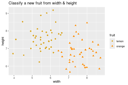
Four ways to draw the boundary
Every classifier we’ve met carves the feature space differently.
- k-nearest-neighbours (kNN) — to label a new point, take its \(k\) nearest training points and let them vote. (\(k = 1\) is the plain nearest-neighbour of the neural networks notes.) The boundary is a patchwork of little islands around clusters of each class.
- Logistic regression — a single straight line (a hyperplane in higher dimensions): one side orange, the other lemon.
- Neural network — logistic regression with a more flexible function: a smooth curved boundary.
- Decision tree — repeatedly split the space in half on one feature at a time, giving a boundary of axis-parallel rectangles.
kNN, concretely
library(class)
set.seed(2)
train_idx <- sample(nrow(fruit), 60)
train <- fruit[train_idx, ]
test  <- fruit[-train_idx, ]

pred <- knn(train = train[, c("width", "height")],
            test  = test[,  c("width", "height")],
            cl    = train$fruit, k = 5)
mean(pred == test$fruit)   # accuracy
## [1] 1kNN needs no “training” beyond storing the data, but it must search all of it at prediction time, and “nearest” uses raw distances, so feature scaling matters.
A decision tree
A tree asks a sequence of yes/no questions. At each internal node a question like “is width > 6.5?” sends you left or right; each leaf gives a label. It looks like an upside-down tree — root at top, leaves at the bottom.
library(rpart)
tree <- rpart(fruit ~ width + height, data = fruit, method = "class")
par(mar = c(1, 1, 1, 1))
plot(tree, margin = 0.1); text(tree, use.n = TRUE, cex = 0.9)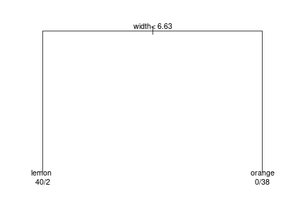
Read a prediction by walking root-to-leaf. Notice a tree may ignore a feature entirely if it isn’t useful, and may split on the same feature more than once at different thresholds. Let’s see the rectangular boundary it induces:
grid <- expand.grid(
  width  = seq(min(fruit$width),  max(fruit$width),  length.out = 200),
  height = seq(min(fruit$height), max(fruit$height), length.out = 200))
grid$pred <- predict(tree, grid, type = "class")

ggplot() +
  geom_tile(data = grid, aes(width, height, fill = pred), alpha = 0.3) +
  geom_point(data = fruit, aes(width, height, color = fruit, shape = fruit), size = 2) +
  scale_fill_manual(values = c(lemon = "goldenrod", orange = "darkorange")) +
  scale_color_manual(values = c(lemon = "goldenrod", orange = "darkorange")) +
  labs(title = "A decision tree splits into axis-parallel rectangles")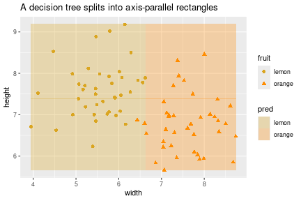
What can a tree represent?
In principle any boolean function of the inputs — including patterns a straight line can’t separate. The classic one is XOR / checkerboard: label \(1\) on two diagonally-opposite corners, \(0\) on the other two.
xor_df <- data.frame(
  x1    = c(0, 0, 1, 1),
  x2    = c(0, 1, 0, 1),
  label = factor(c(0, 1, 1, 0)))
xor_df
## x1 x2 label
## 1 0 0 0
## 2 0 1 1
## 3 1 0 1
## 4 1 1 0No straight line separates the two labels, so logistic regression fails here — but a small tree handles it easily (split on x1, then on x2 within each half).
A caveat about that intuition, though: in two dimensions lots of things aren’t linearly separable, but with many features (say 50), a separating hyperplane usually does exist — our 2-D geometric intuition misleads us. So logistic regression works far more often than the XOR picture suggests.
The flip side: some simple-looking functions are hard for trees. The parity function (output 1 iff an odd number of inputs are 1) is a high-dimensional checkerboard; a tree can represent it but needs to split on every feature repeatedly, so it takes a large tree and lots of data. As you allow bigger trees (more nodes, more depth), the hypothesis space — the set of labelings the tree can express — grows; logistic regression’s is always just “which hyperplane?”
How a tree is learned
Finding the optimal tree is NP-hard, so in practice we use a greedy heuristic: grow the tree top-down, at each step picking the split that looks best right now, then recurse on each side.
learn(data):
  if all labels in `data` are the same -> make a leaf
  else:
    pick the feature (and threshold) whose split is "best"
    partition data into S0, S1 by that split
    learn(S0); learn(S1)      # recurse on each side
Details:
- Discrete feature → one branch per category. Continuous feature → pick a threshold. You don’t try every real number: only values present in the data can matter, so you try thresholds between adjacent observed values.
- Which split is “best”? Simplest: try each feature’s best threshold and take the one giving the lowest error rate, where a not-yet-pure node is labeled by majority vote. One subtlety — error count can stay the same after a useful split, so real implementations use an information-theoretic score (information gain / Gini) instead of raw error. Same idea, more sensitive.
Random forests
A single tree is easy to overfit and sensitive to the data. The fix that dominates tabular-data competitions (e.g. on Kaggle) is the random forest: grow many trees — each on a random resample of the data and a random subset of features — and average their predictions. Many trees ⇒ a “forest” (the name is a mild joke). You rarely build these by hand; a library does it. Empirically, for a plain table of features with labels, a random forest is often the most accurate off-the-shelf choice.
Interpretability
Trees are often sold as interpretable: you can read the learned tree and say “outlook matters most; if it’s sunny, then humidity matters.” True for a small tree. But two caveats: a tree past a few branches is hard to hold in your head, and because it was built greedily, the feature at the root isn’t guaranteed to be the genuinely most important one. And a random forest — an average of many trees — loses this transparency almost entirely. So “interpretable” is real but limited.
Summary
- kNN: vote among the \(k\) nearest training points; boundary is islands; no training, but stores and searches all data.
- Classifiers carve space differently — line (logistic regression), smooth curve (neural net), axis-parallel rectangles (tree), islands (kNN).
- A decision tree asks yes/no questions down to leaf labels; it can represent any boolean function (including XOR, which defeats a linear model), but some functions (parity) need a huge tree.
- Trees are learned greedily (optimal is NP-hard): pick the best split, recurse; thresholds come from values in the data; score splits by information gain.
- Random forests — averages of many trees — are the go-to for tabular data, trading interpretability for accuracy.
References
- Builds on neural networks (nearest-neighbour, the model comparison) and logistic regression (the linear boundary).
- Hastie, Tibshirani & Friedman, The Elements of Statistical Learning, Ch. 9 (trees) and Ch. 15 (random forests).