18.7 Running-Time Analysis for Mergesort and Quicksort

In the past two sections, we introduced two recursive sorting algorithms, mergesort and quicksort. We’ll now analyse the running time of these two algorithms, which will use the same technique that we introduced in 15.4 Running-Time Analysis for Tree Operations. As a reminder before we begin, here is the approach we use for this type of running-time analysis:

Find a pattern for the (tree) structure of recursive calls made for our recursive function.
Analyse the non-recursive running time of the recursive calls. Remember that this means counting all recursive calls as constant time, or one step.
“Fill in the tree” of recursive calls with the non-recursive running time, and then add up all of these numbers to obtain the total running time.

Analysing mergesort

Recall the mergesort algorithm:

def mergesort(lst: list) -> list:
    if len(lst) < 2:
        return lst.copy()  # Use the list.copy method to return a new list object
    else:
        # Divide the list into two parts, and sort them recursively.
        mid = len(lst) // 2
        left_sorted = mergesort(lst[:mid])
        right_sorted = mergesort(lst[mid:])

        # Merge the two sorted halves. Using a helper here!
        return _merge(left_sorted, right_sorted)

Let’s now analyse the running time of this algorithm. First we need to analyse the structure of the recursive calls made. Suppose we start with a list of length $n$ , where $n > 1$ . For simplicity, we’ll assume that $n$ is a power of 2. The analysis we’ll do in this section applies to when $n$ isn’t a power of two, but is trickier because the list isn’t always divided into two exactly equal halves. In the recursive step, we divide the list in half, obtaining two lists of length $\frac{n}{2}$ , and recurse on each one. Each of those calls divides their list in half, obtaining and recursing on lists of length $\frac{n}{4}$ . This pattern repeats, with each call to mergesort taking as input a list of length $\frac{n}{2^{k}}$ (for some $k \in N$ ) and recursing on two lists of length $\frac{n}{2^{k + 1}}$ . The base case is reached when mergesort is called on a list of length 1.

For example, here are the lists that would be passed as inputs to mergesort from an initial call to mergesort on the list [3, -1, 7, 10, 6, 2, -3, 0].

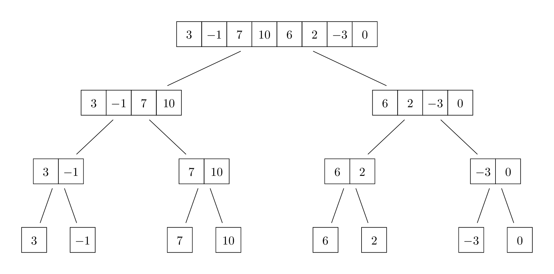
Mergesort recursion diagram example.

In other words, our recursive call diagram is a binary tree: every non-base-case call to mergesort makes two more recursive calls, one of the left half of its input and one on the right half. But that’s not all: because we know that the input list decreases in size by a factor of 2 at each recursive call, we know what the height of the tree is. If we start with an input list of height $n$ , where $n$ is a power of 2, there are exactly $\log_{2} (n) + 1$ levels in this tree. The $+ 1$ might look a bit funny, but you can confirm this with the above diagram, where $n = 2^{3}$ .

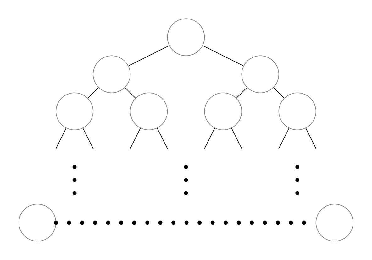
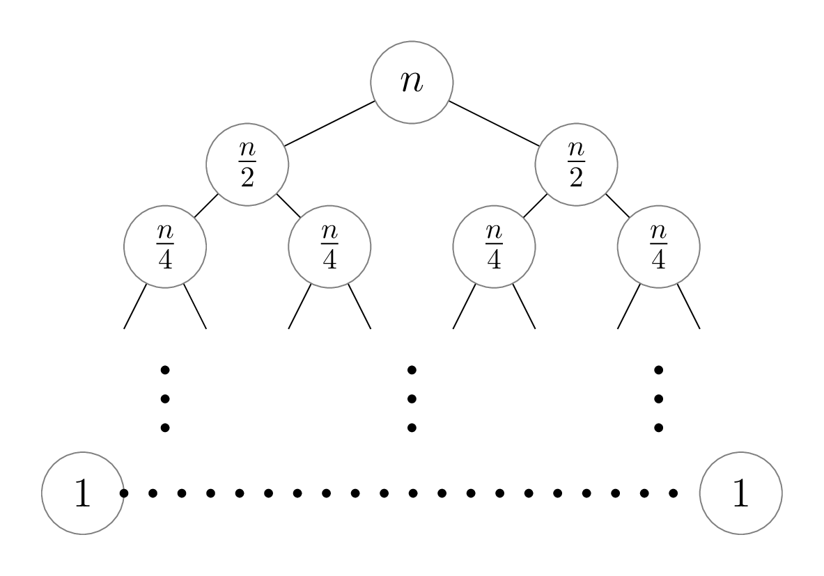
So in general our recursion diagram for mergesort looks like this:

Non-recursive running time

Next, let’s analyse the non-recursive running time of mergesort. Consider a list lst of length $n$ , where $n \geq 2$ . Again, we’ll assume $n$ is a power of 2, which allows us to ignore floors/ceilings in our calculation. In this case:

The if condition check (len(lst) < 2) and calculation of mid take constant time.
The list slicing operations lst[:mid] and lst[mid:] each take time proportional to the length of the slice, which is $\frac{n}{2}$ .Note that while this slicing occurs in the same line as a recursive call, the slicing itself is considered non-recursive, since it occurs before making the recursive calls.
We’ll leave the running-time analysis of _merge as an exercise, but the running time is $Θ (n_{1} + n_{2})$ , where $n_{1}$ and $n_{2}$ are the sizes of its two input lists.

So in the recursive step, left_sorted and right_sorted each have size $\frac{n}{2}$ , the running time of _merge(left_sorted, right_sorted) is $\frac{n}{2} + \frac{n}{2} = n$ steps.

So the total non-recursive running time of mergesort is $1 + \frac{n}{2} + \frac{n}{2} + n = 2 n + 1$ , when $n \geq 2$ .

(Note: when $n < 2$ , the base case executes, which is constant time. We count that as 1 step.)

Putting it all together

Now that we have this non-recursive running time, we can fill in our recursion tree. We’re going to make another simplification to our analysis: we’ll use $n$ instead of $2 n + 1$ as the running time, essentially taking the “simplified Theta bound” of the previous expression. This is different than the previous recursive running-time analyses we did for trees! We’re doing it here just to make the calculation work out nicely, but rest assured that if we used the $2 n + 1$ expression we’d get the same Theta bound at the end. So what we get is the following:

The initial mergesort call on a list of length $n$ takes $n$ steps.
Each of the recursive mergesort calls on a list of length $\frac{n}{2}$ takes $\frac{n}{2}$ steps.
Then, each of the recursive mergesort calls on a list of length $\frac{n}{4}$ takes $\frac{n}{4}$ steps.
This pattern continues, until we reach our base case (list of length 1), which takes 1 step.

Mergesort recursion diagram with filled nodes.

Okay, so we’ve filled in our tree; the last remaining step is to add up all of the numbers. This might look daunting at first, since we have several different numbers to add up, so we can’t simply multiply the number of nodes by the non-recursive running time of a single one.

Here is our key observation: each level in the tree has nodes with the same running time, and since this is a binary tree we can find a simple formula for the number of nodes at any depth in the tree. More precisely, at depth $d$ in the tree, there are $2^{d}$ nodes, and each node contains the number $\frac{n}{2^{d}}$ . Remember, depth starts at 0, so the tree’s root has depth 0. So when we add up the nodes at each depth, we get $2^{d} \cdot \frac{n}{2^{d}} = n$ . In other words, each level in the tree has the same total running time!

Now we can use our previous observation that there are $\log_{2} (n) + 1$ levels in total to obtain a total running time of $n \cdot (\log_{2} (n) + 1)$ , which is $Θ (n \log n)$ . So after all that work, we do get something quite special: the running time of mergesort is much better than the $Θ (n^{2})$ (worst-case) running times of selection sort and insertion sort. Hooray for recursion!

Quicksort: how quick is it?

Now let’s turn our attention to quicksort. Is it possible to do the same running-time analysis that we did for mergesort? Not quite.

def quicksort(lst: list) -> list:
    if len(lst) < 2:
        return lst.copy()
    else:
        # Partition the list using the first element as the pivot
        pivot = lst[0]
        smaller, bigger = _partition(lst[1:], pivot)

        # Sort each part recursively
        smaller_sorted = quicksort(smaller)
        bigger_sorted = quicksort(bigger)

        # Combine the two sorted parts. No need for a helper here!
        return smaller_sorted + [pivot] + bigger_sorted

First let’s start with the parts that are similar. The non-recursive running time of quicksort is also $Θ (n)$ , where $n$ is the length of the input list. We’ll leave the exact running-time this as a good exercise to do. Note that even though the list slicing lst[1:] is relatively inefficient, it still just takes $Θ (n)$ time. The other similarity is that quicksort also always makes two recursive calls, on its two partitions. Because of this, the recursive call tree is also a binary tree.

The key difference is that with mergesort we know that we’re splitting up the list into two equal halves (each of size $\frac{n}{2}$ ); this isn’t necessarily the case with quicksort!

Suppose we get lucky, and at each recursive call we choose the pivot to be the median of the list, so that the two partitions both have size (roughly) $\frac{n}{2}$ . In this case, the recursion tree is the same as mergesort, and we get a $Θ (n \log n)$ runtime.

But this relies on making an assumption about our choice of pivot. Consider another possibility: what if we’re always extremely unlucky, and always choose the smallest list element? In this case, the partitions are as uneven as possible, with smaller having no elements, and bigger having all remaining $n - 1$ elements. This results in a very lopsided recursion diagram, with the following non-recursive running times: Note that the “1” nodes down the tree represent the running time of making the recursive calls on an empty list.

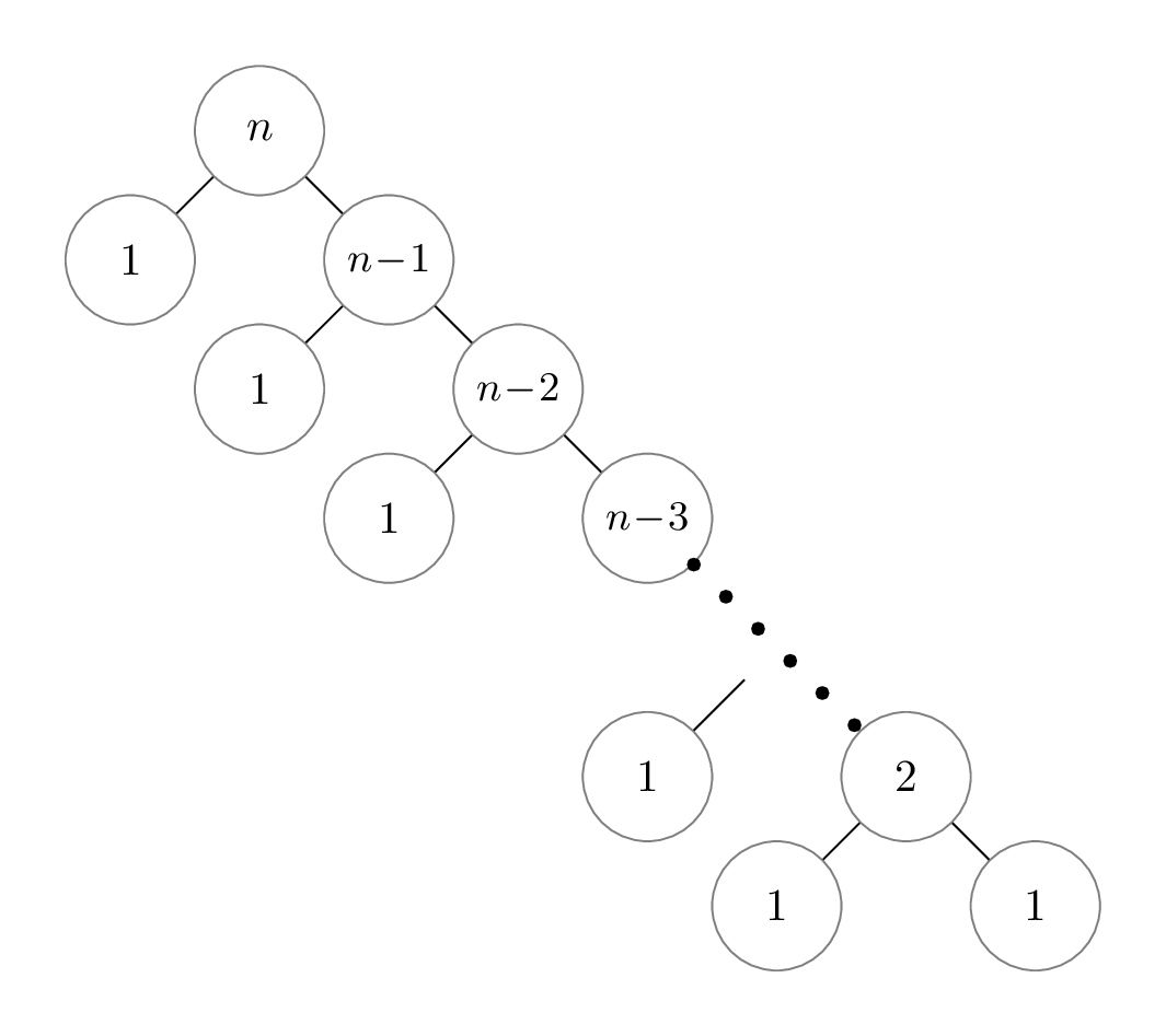
Unbalanced quicksort running time tree

In this case, the height of the tree is $n$ , since the size of the bigger partition just decreases by 1 at each call. There are $n - 1$ recursive calls on empty partitions (smaller). Adding the total non-recursive running time gives us:

$(\sum_{i = 1}^{n} i) + (n - 1) = \frac{n (n + 1)}{2} + n - 1$

And so for this case, the running time is actually $Θ (n^{2})$ , just like selection sort and insertion sort!

In fact, these two cases mark the extremes of the running time ranges for quicksort. It’s possible to show (with a more formal analysis) that the worst-case running time for this implementation of quicksort is $Θ (n^{2})$ , and the best-case (i.e., minimum) running time is $Θ (n \log n)$ . So it seems like quicksort isn’t actually so quick after all, at least in the worst case. The choice of pivot is extremely important, because if we repeatedly choose pivots that result in uneven partitions, the running time increases significantly. In our naive implementation of quicksort, where the first list item is chosen as the pivot, this actually means that getting an already-sorted list as input results in this poor $Θ (n^{2})$ running time—not great!

Mergesort and quicksort in practice

Given the running-time analyses of mergesort and quicksort we’ve done in the previous section, you might wonder whether quicksort why quicksort would ever be used over mergesort. In practice, however, there are a few complexities that make things less clear cut.

The main strength of asymptotic Theta notation is that is simplifies our running-time analyses, so that we don’t need to worry about getting constant factors exactly right. But this same simplification also has the effect of flattening reported running times, so that all $Θ (n \log n)$ times look the same. In practice, an in-place implementation of quicksort can be significantly faster than mergesort: for most inputs, quicksort has “smaller constants” than mergesort, and performs fewer primitive machine operations than mergesort does. Simply put, for most inputs quicksort is faster than mergesort, even though its worst-case running time is larger.

In fact, with some more background in probability theory, we can talk about the performance of quicksort on a random list of length $n$ , or equivalently, what happens when we always choose a random element to be the pivot in the partitioning step. This leads to a different form of running-time analysis known as average-case running time analysis. We can prove that quicksort has an average-case running time of $Θ (n \log n)$ —with smaller constant factors than mergesort’s $Θ (n \log n)$ —which indicates that the actual “bad” inputs for quicksort are quite rare. Doing an average-case running time analysis of quicksort is a common example used in CSC263/265!

There are some other interesting points we’ll make before wrapping up. The first is that there actually exists a linear-time algorithm for computing the median of a list of numbers.This is known as the median of medians algorithm, which we encourage you to look up! This means that we can always choose the median of the list as the pivot in quicksort’s partitioning step, making the worst-case running time $Θ (n \log n)$ . However, even though this version of quicksort has a better worst-case running time, the extra steps used to calculate the median typically results in a slower running time for more inputs than simply choosing a random pivot. In practice, this version of quicksort is rarely used.

And finally, we would be remiss if we didn’t answer the question that must be on your mind: what sorting algorithm do Python’s built-in sorted and list.sort functions use?! It turns out that Python uses a sorting algorithm known as Timsort, which was invented by Tim Peters in 2002 specifically for the Python programming language. You might be disappointed that we didn’t cover that algorithm in this course, but in fact, Timsort is essentially a highly optimized version of mergesort. Timsort uses the same basic idea of merging sorted sublists, but does so in a much smarter and more efficient way than our mergesort implementation, and adds a few tweaks based on empirical tests. One of those tweaks is switching to insertion sort to sort small sublists, which again reveals how our asymptotic worst-case running time doesn’t tell the full story.