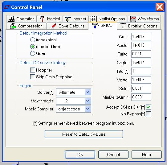
First, set ltspice to be more accurate. In the menu, choose Simulate->Control Panel, then choose the "Spice" tab. See the image below.
Set the Solver to Alternate. For higher accuracy set Reltol to a smaller number. The smaller it is, the slower the simulation will run.

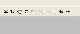
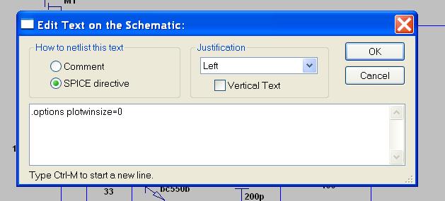
It helps with accuracy to also set the compression to zero. Click on the .op button, upper right.

Type ".options plotwinsize=0" in the dialogue.

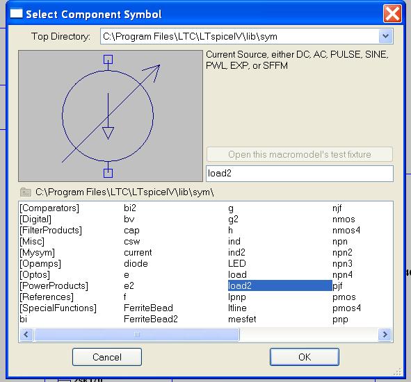
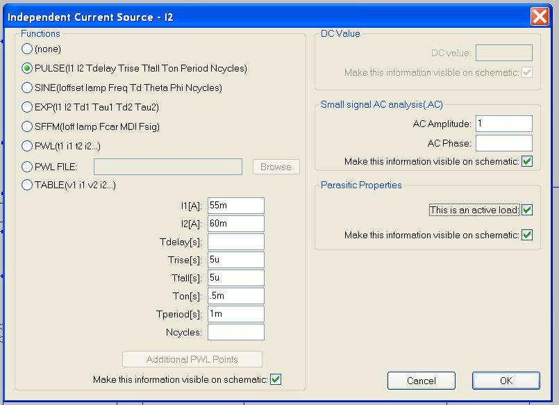
To create an output impedance bode plot, a load needs to be inserted at the output of the system. Select Edit->Component (or press F2), and you will get the Select component dialog. I usually choose load2, and put it in the circuit.

Once in the circuit, click the right button mouse on it and you should get the Independent Current Source settings dialog. For the output impedance plot it does not matter what is chosen under "Functions." However, under "Small signal AC analysis (AC)," the AC Amplitude should be set to 1. Similarly, it does not matter what is chosen under "Small signal..." for a .trans analysis, but it matters what you choose under "Functions."

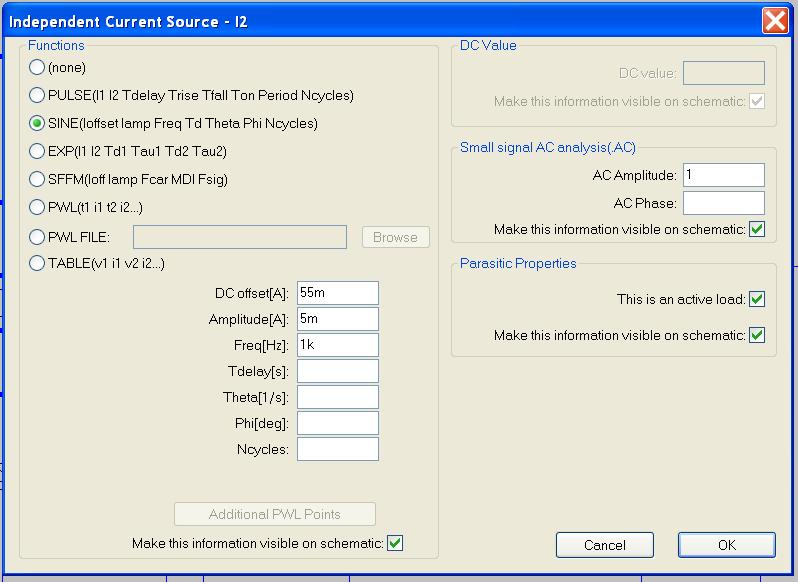
Just another example of choose a sine wave function as the load. Again, this does not change anything in the output impedance plot.

Next, choose Simulate->Edit simulation cmd, and click on the "AC Analysis" tab. See the image below for an example.

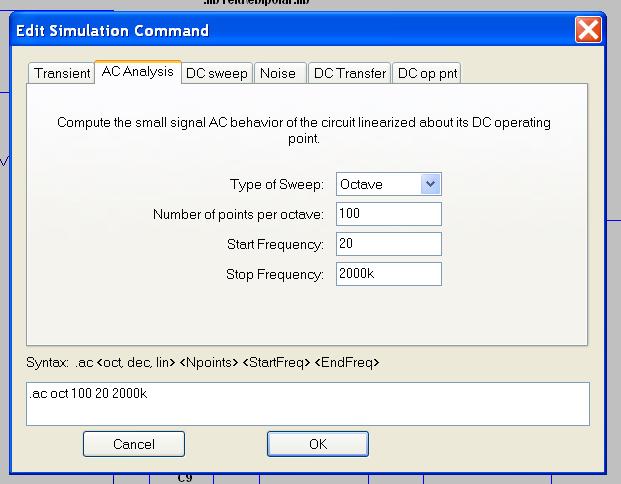
When you click on OK, the first time you do this your mouse pointer will have the command stuck to it, and you have to place it somewhere on the screen, next to the circuit. You're now ready to run the simulation: either choose from the menu Simulate->Run or click on the "running man" button in the toolbar. This will open a window. Click with the left button mouse on the trace of interest, usually the output, right above the load. A plot will be drawn, with the Y axis in decibels, and the X axix in hertz.

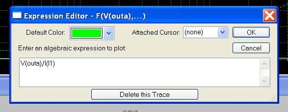
For output impedance, first let's set the Y axis to linear. Click the left mouse button to the left of the Y axis, where the db values are written. In the dialogue that opens, choose "linear" and click on OK. This will change the shape of the plot, and the units on the Y axis to volts. You can consider the values as ohms, since the magnitude is right. However, to not confuse fellow diyers, it is nice to post impedance plots in ohms. Let's assume you assigned the label "outa" to the output trace that was ploted. To get ohms on the Y axis, in the plot, click the right mouse button on the V(outa) label, at the top of the plot. In the dialogue, after "V(outa)" type "/I(I1)" and press OK. This assumed that the load is named I1, but in your case it may be I2, or I3, or whatever. The idea is that you divide the output voltage by the output current, V/I to get impedance in ohms.

Another thing that might help in analyzing the impedance easier is to zoom in on a range of the Y axis. Click the left mouse button on the left of the Y axis again, and set the top range whatever interests you, like 2m (that would be two milliohms), bottom range to 0m, and the tick mark to .1m for instance (100 microohms). Then press OK. If you don't see the grid on the plot and you'd like to, press CTRL-G. on the plot,