How many modes can a Gaussian mixture have?

One problem I considered during my PhD thesis was that of reconstructing a sequence with missing data. I approached it by defining multivalued mappings via Gaussian-mixture conditional distributions, where the M modes of a conditional distribution p(y|x=x0) represent the values f(x0) = {y1,...,yM} (the sequence was then reconstructed by dynamic programming minimisation of a continuity constraint on those values). This led me to develop algorithms for finding the modes and to consider the question how many modes does a Gaussian mixture with M components have? I conjectured that Gaussian mixtures with isotropic components could have no more modes than components. Work by myself, Chris Williams and others has now resolved this conjecture; see below for the cases when it holds. For more details, and algorithms for mode-finding, see the references at the bottom of this page.

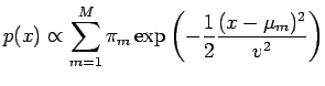
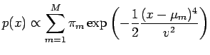
Assume a Gaussian-mixture probability density function p(x) in D dimensions, given by

This mixture has M components, each with its own weight, centroid and covariance (π, μ, Σ, respectively).

Dimension D = 1: a Gaussian mixture with M components can have at most M modes

This can be proven using results from scale-space theory (see CarreirWilliam03a). Furthermore, no other type of mixture (i.e., with kernels other than the Gaussian) has this property. Click on the following to see animations of 1D mixtures:

• 
  1D mixture of Gaussians: the density is plotted for a range of values of the scale v in the upper graph of the animation. The location of the maxima (blue) and minima (red) is tracked in the lower graph. Note how as the scale increases no new maxima are created: the only events that can happen are annihilations of a pair maximum-minimum. The number of modes is equal to the number of components for small scale and decreases as the scale increases.
• 
  1D mixture of non-Gaussian kernels: here we do the same but using a kernel exp(-0.5*x^4/v^2) instead of the Gaussian kernel exp(-0.5*x^2/v^2). Note how as the scale increases new maxima are created: we can have events both of annihilation and creation. The number of modes can be larger than the number of components.

Dimension D > 1: a Gaussian mixture with M components can have more than M modes

If the components are not isotropic, it is easy to find examples with more modes than components. For example, consider the following one in D = 2. Left contour plot: M = 2 components, 3 modes. Right contour plot: M = 6 components, 9 modes. The thick line is the convex hull of the component centroids, the + (cross) are the centroids and the ∆ (triangle) are the modes.

If the components are isotropic, it is very hard to find examples with more modes than components. Prof. J. J. Duistermaat (pers. comm., 2003) found the following one in 2D. It consists of 3 components, lying at the vertices of an equilateral triangle (here with unit circumcircle radius), with the same, round covariance (of radius v). For a narrow interval [0.707,0.739] of the variance v, a fourth mode exists at the triangle centre. Click on the picture to see an animation for a range of variances (the modes lie at the crosses +). Note how, as v increases from 0, the 3 modes at the vertices (and 3 corresponding saddle points at the midpoint of the sides) move towards the centre, which starts as a minimum. At v = 0.707 the saddles merge with the minimum at the centre; the result is that the centre becomes a maximum and 3 other saddles appear that travel away from the centre towards the vertices; we now have 4 modes. At v = 0.739 the maxima from the vertices annihilate with the saddles at a distance 0.377 from the centre and we end up with a single maximum. The region around the modes when there are 4 modes is very flat; to show the modes, I have had to add many contours at manually selected levels.
View it as a high-quality animation (gzip-compressed lossless AVI) , as a low-quality animation (AVI) or as a low-quality animation (MPEG) .

This example doesn't seem to hold for a polygon other than the triangle. However, it carries over to D > 2 dimensions as a simplex; the variance interval length peaks at D = 699 and decreases very slowly towards 0 as D goes to infinity.

Thus, a Gaussian mixture in 2D or higher can have more modes than components. However, this is a rare occurrence.

Software

The modes of a Gaussian mixture don't have a closed-form expression, so they have to be found numerically by iterative methods. One approach I followed (Carreir00a) is to start a hill-climbing search from the centroid of every component; in practice, this usually finds all the modes (if, as seen above, there are more modes than components, it will miss some, of course). The following Matlab software implements some of the algorithms for mode-finding in Gaussian mixtures (including the calculation of error bars, gradient and Hessian at each mode).

The following images show one of the algorithms in action for an isotropic Gaussian mixture. This algorithm is a fixed-point iteration that can be seen as an EM algorithm; the mixture density p(x) is in fact a likelihood surface whose local maxima are the modes of the Gaussian mixture. The mean shift algorithm of Fukunaga and Hostetler, 1975 for isotropic Gaussian kernels is a particular case of this algorithm. Left contour plot: centroids (+), modes (∆), convex hull of centroids (thick line polygon; the modes must lie inside for isotropic components); the grey circles represent the components. Right contour plot: sequences of iterates of the algorithm, starting from each centroid and converging to the modes. The light/dark areas indicate negative/positive Hessian of p(x), respectively.

The following picture shows, for a different isotropic Gaussian mixture, the sequence of iterates and uses colours to mark the domains of convergence to each mode (there are 4 modes). Note how these domains may be nonconvex and disconnected (this also demonstrates that the domains of convergence of an EM algorithm to the local maxima of a log-likelihood surface may be nonconvex and disconnected).

References

• [Carreir00a] Carreira-Perpinan, M. A. (2000): "Mode-finding for mixtures of Gaussian distributions". IEEE Trans. on Pattern Analysis and Machine Intelligence 22(11): 1318-1323.
  [External link] [paper preprint] [© IEEE] [Matlab implementation]
  Extended technical report version:
  Carreira-Perpinan, M. A. (1999): Mode-finding for mixtures of Gaussian distributions (revised August 4, 2000). Technical report CS-99-03, Dept. of Computer Science, University of Sheffield, UK.
  [External link] [paper]

• [Carreir01a] Carreira-Perpinan, M. A. (2001): Continuous latent variable models for dimensionality reduction and sequential data reconstruction. PhD thesis, University of Sheffield, UK.
  Chapter 8 deals with mode-finding in Gaussian mixtures, while chapter 7 describes a sequential data reconstruction approach where mode-finding algorithms are useful.

• [CarreirWilliam03a] Carreira-Perpinan, M. A. and Williams, C. K. I. (2003): On the number of modes of a Gaussian mixture. Technical report EDI-INF-RR-0159, School of Informatics, University of Edinburgh, UK.
  [External link] [paper]
  A shortened version appeared as:
  Carreira-Perpinan, M. A. and Williams, C. K. I. (2003): "On the number of modes of a Gaussian mixture" (2003). Scale-Space Methods in Computer Vision, pp. 625-640, Lecture Notes in Computer Science vol. 2695, Springer-Verlag.
  [External link] [paper preprint] [© Springer-Verlag]

• [CarreirWilliam03b] Carreira-Perpinan, M. A. and Williams, C. K. I. (2003): An isotropic Gaussian mixture can have more modes than components. Technical report EDI-INF-RR-0185, School of Informatics, University of Edinburgh, UK.
  [External link] [paper]

University of Toronto | Dept. of Computer Science | Machine learning group | MACP's Home Page |