1	Learning Energy-Based Models of High-Dimensional Data Geoffrey Hinton Max Welling Yee-Whye Teh Simon Osindero
2	Discovering causal structure as a goal for unsupervised learning It is better to associate responses with the hidden causes than with the raw data. The hidden causes are useful for understanding the data. It would be interesting if real neurons really did represent independent hidden causes.
3	A different kind of hidden structure Instead of trying to find a set of independent hidden causes, try to find factors of a different kind. Capture structure by finding constraints that are Frequently Approximately Satisfied. Violations of FAS constraints reduce the probability of a data vector. If a constraint already has a big violation, violating it more does not make the data vector much worse (i.e. assume the distribution of violations is heavy-tailed.)
4	Two types of density model Stochastic generative model using directed acyclic graph (e.g. Bayes Net) Synthesis is easy Analysis can be hard Learning is easy after analysis Energy-based models that associate an energy with each data vector Synthesis is hard Analysis is easy Is learning hard?
5	Bayes Nets It is easy to generate an unbiased example at the leaf nodes. It is typically hard to compute the posterior distribution over all possible configurations of hidden causes. Given samples from the posterior, it is easy to learn the local interactions
6	Approximate inference What if we use an approximation to the posterior distribution over hidden configurations? e.g. assume the posterior factorizes into a product of distributions for each separate hidden cause. If we use the approximation for learning, there is no guarantee that learning will increase the probability that the model would generate the observed data. But maybe we can find a different and sensible objective function that is guaranteed to improve at each update.
7	A trade-off between how well the model fits the data and the tractability of inference This makes it feasible to fit very complicated models, but the approximations that are tractable may be very poor.
8	Energy-Based Models with deterministic hidden units Use multiple layers of deterministic hidden units with non-linear activation functions. Hidden activities contribute additively to the global energy, E.
9	Maximum likelihood learning is hard To get high log probability for d we need low energy for d and high energy for its main rivals, c
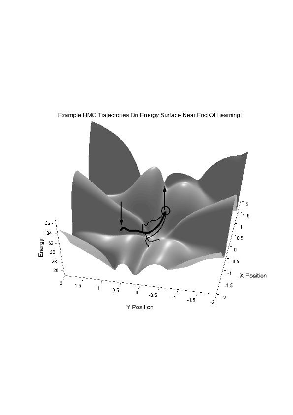
10	Hybrid Monte Carlo The obvious Markov chain makes a random perturbation to the data and accepts it with a probability that depends on the energy change. Diffuses very slowly over flat regions Cannot cross energy barriers easily In high-dimensional spaces, it is much better to use the gradient to choose good directions and to use momentum. Beats diffusion. Scales well. Can cross energy barriers.
11
12	Backpropagation can compute the gradient that Hybrid Monte Carlo needs Do a forward pass computing hidden activities. Do a backward pass all the way to the data to compute the derivative of the global energy w.r.t each component of the data vector. works with any smooth non-linearity
13	The online HMC learning procedure Start at a datavector, d, and use backprop to compute for every parameter. Run HMC for many steps with frequent renewal of the momentum to get equilbrium sample, c. Use backprop to compute Update the parameters by :
14	A surprising shortcut Instead of taking the negative samples from the equilibrium distribution, use slight corruptions of the datavectors. Only add random momentum once, and only follow the dynamics for a few steps. Much less variance because a datavector and its confabulation form a matched pair. Seems to be very biased, but maybe it is optimizing a different objective function. If the model is perfect and there is an infinite amount of data, the confabulations will be equilibrium samples. So the shortcut will not cause learning to mess up a perfect model.
15	Intuitive motivation It is silly to run the Markov chain all the way to equilibrium if we can get the information required for learning in just a few steps. The way in which the model systematically distorts the data distribution in the first few steps tells us a lot about how the model is wrong. But the model could have strong modes far from any data. These modes will not be sampled by confabulations. Is this a problem in practice?
16	Contrastive divergence Aim is to minimize the amount by which a step toward equilibrium improves the data distribution.
17	Contrastive divergence .
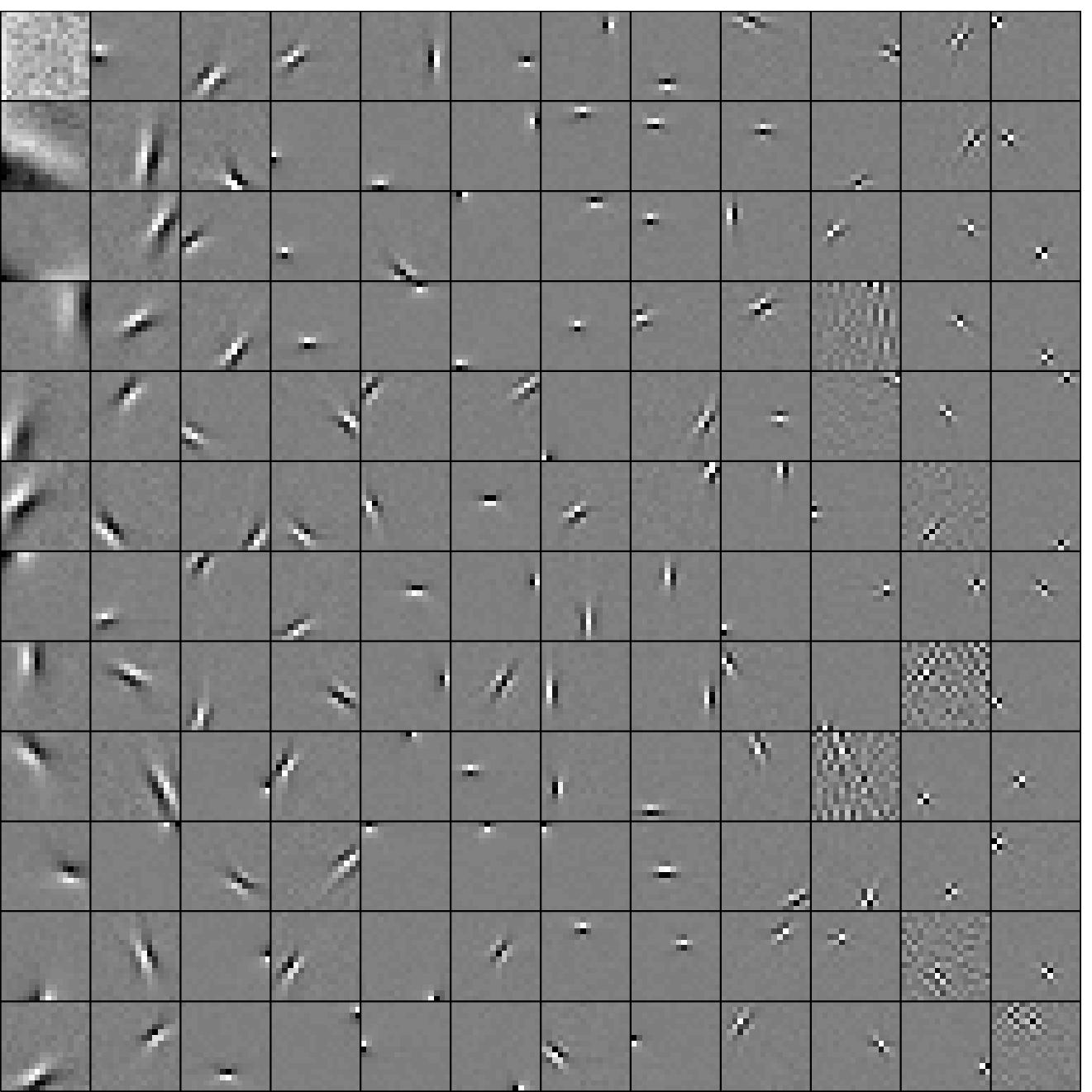
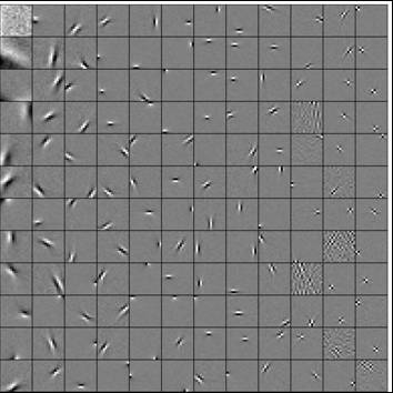
18	Frequently Approximately Satisfied constraints The intensities in a typical image satisfy many different linear constraints very accurately, and violate a few constraints by a lot. The constraint violations fit a heavy-tailed distribution. The negative log probabilities of constraint violations can be used as energies.
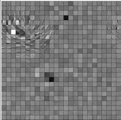
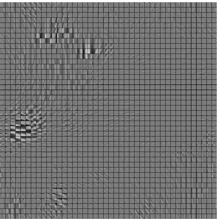
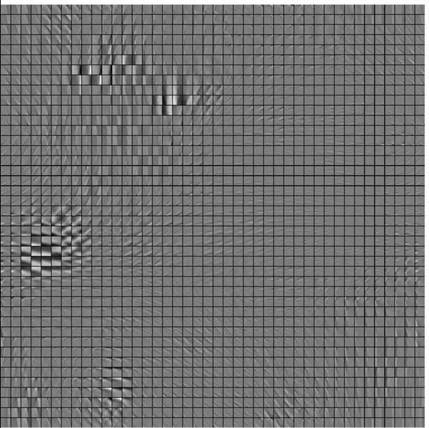
19	Learning constraints from natural images (Yee-Whye Teh) We used 16x16 image patches and a single layer of 768 hidden units (3 x overcomplete). Confabulations are produced from data by adding random momentum once and simulating dynamics for 30 steps. Weights are updated every 100 examples. A small amount of weight decay helps.
20
21
22	How to learn a topographic map
23
24	Faster mixing chains Hybrid Monte Carlo can only take small steps because the energy surface is curved. With a single layer of hidden units, it is possible to use alternating parallel Gibbs sampling. Much less computation Much faster mixing Can be extended to use pooled second layer (Max Welling) Can only be used in deep networks by learning one hidden layer at a time.
25
26
27