CSC411 Project 2: Deep Neural Networks for Handwritten Digit and Face Recognition 
For this project, you will build several neural networks of varying depth, and use them for handwritten digit recognition and face recognition. You may import things like numpy and matplotlib, but the idea is to implement things “from scratch”: you may not import libraries that will do your work for you, unless otherwise specified. You should only use PyTorch for face recognition.
The input: digits
For parts 1-6 you will work with the MNIST dataset. The dataset is available in easy-to-read-in format here, with the digits already seprated into a training and a test set. I recommend you divide the data by 255.0 (note: the .0 is important) so that it’s in the range 0..1.
Handout code: digits
We are providing some code here (data: snapshot50.pkl. You need to read it using pickle.load(open("snapshot50.pkl", "rb"), encoding="latin1") in Python 3).
The code provides a partial implementation of a single-hidden-layer neural network with tanh activation functions in the hidden layer that classifies the digits. The code is not meant to be run as is. We are simply providing some functions and code snippets to make your life easier.
Part 1 (2 pts)
Describe the dataset of digits. In your report, include 10 images of each of the digits. You may find matplotlib’s subplot useful for displaying multiple images at once.
Part 2 (3 pts)
Implement a function that computes the network below using NumPy (do not use PyTorch for parts 1-6).
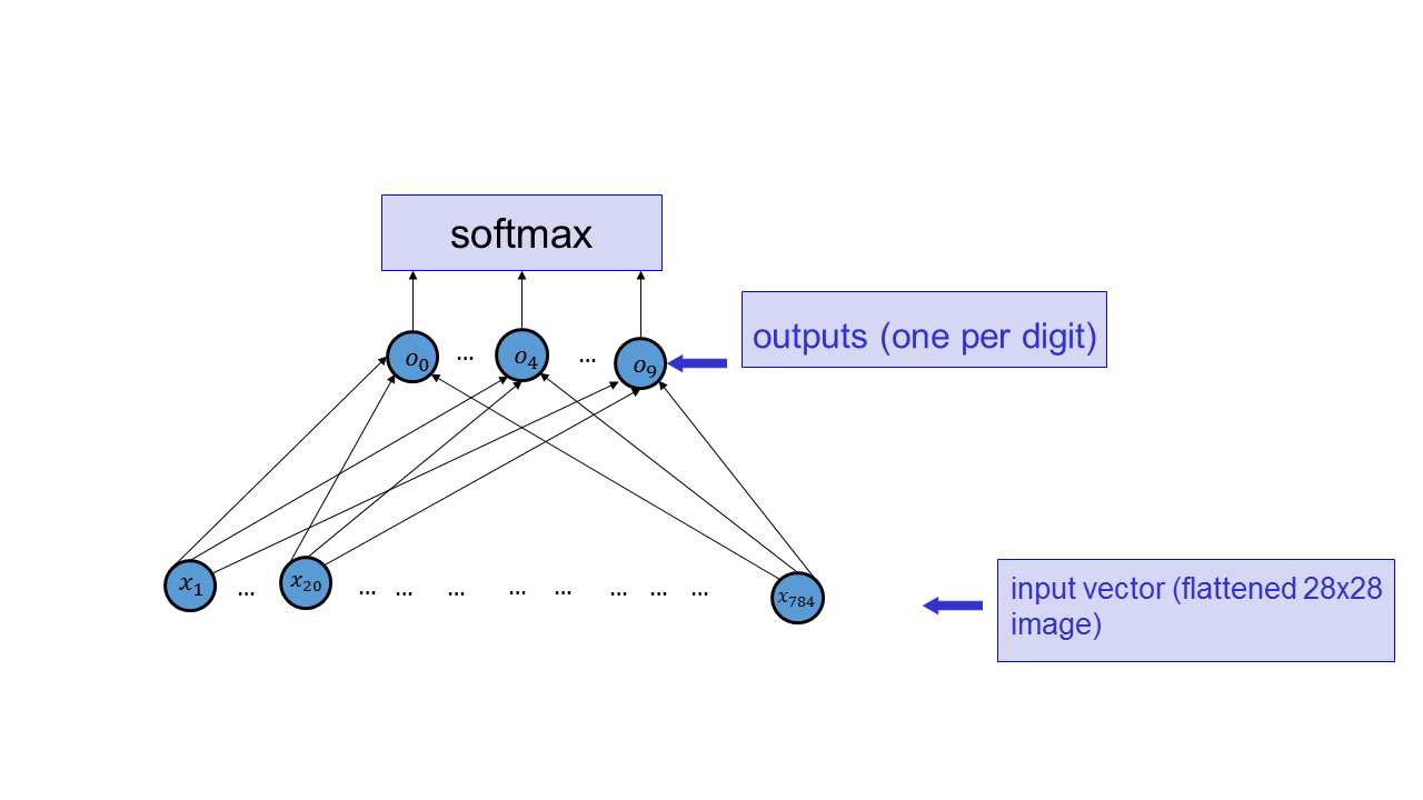
The \(o\)’s here should simply be linear combinations of the \(x\)’s (that is, the activation function in the output layer is the identity). Supecifically, use \(o_i = \sum_j w_{ji} x_j + b_i\). Include the listing of your implementation (i.e., the source code for the function; options for how to do that in LaTeX are here) in your report for this Part.
Part 3 (10 pts)
We would like to use the sum of the negative log-probabilities of all the training cases as the cost function.
Part 3(a) (5 pts)
Compute the gradient of the cost function with respect to the weight \(w_{ij}\). Justify every step. You may refer to Slide 7 of the One-Hot Encoding lecture, but note that you need to justify every step there, and that your cost function is the sum over all the training examples.
Part 3(b) (5 pts)
Write vectorized code that computes the gradient of the cost function with respect to the weights and biases of the network. Check that the gradient was computed correctly by approximating the gradient at several coordinates using finite differences. Include the code for computing the gradient in vectorized form in your report.
Part 4 (10 pts)
Train the neural network you constructed using gradient descent (without momentum). Plot the learning curves. Display the weights going into each of the output units. Describe the details of your optimization procedure – specifically, state how you initialized the weights and what learning rate you used.
Part 5 (5 pts)
In Part 4, we used “vanilla” gradient descent, without momentum. Write vectorized code that performs gradient descent with momentum, and use it to train your network. Plot the learning curves. Describe how your new learning curves compare with gradient descent without momentum. In your report, include the new code that you wrote in order to use momentum.
Part 6 (15 pts)
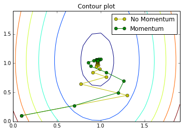
In this Part, you will produce a demonstration of gradient descent working better when momentum is used. From your trained network from Part 5, you should pick two weights. Denote them \(w_1\) and \(w_2\). you will be keeping all other weights constant except \(w_1\) and \(w_2\). To get reasonable results, we recommend that you pick weights associated with the center of the digits, and not along the edges. This is because pixels too close to the edge will likely be black for all digits, and therefore not interesting.
The visualizations you produce in Parts 6(b) and 6(c) should demontrate the benefits of using momentum.
Part 6(a) (4 pts)
Produce a contour plot of the cost function, when the weights \(w_1\) and \(w_2\) are allowed to vary around the values that you obtained in Part 5. Plot the contour of the cost function. The cost function will be a function of the two weights. The two weights \(w_1\) and \(w_2\) should vary around the value obtained in part 5. Label your axes.
Part 6(b) (2 pts)
Re-initialize \(w_1\) and \(w_2\) to a value away from the local optimum. Keeping all other weights constant, learn \(w_1\) and \(w_2\) by taking K steps using vanilla gradient descent (without momentum). Plot the trajectory. You may wish to increase your learning rate from earlier parts so that the number of steps K is not large (say, 10-20).
Part 6(c) (2 pts)
Repeat the experiment, resetting \(w_1\) and \(w_2\) to the same initial value you used in part (b). Now, take K steps using gradient descent with momentum. Plot the trajectory. You do not have to use the same learning rate as in part (b).
Part 6(d) (2 pts)
Describe any differences between the two trajectories. Provide an explanation of what caused the differences.
Part 6(e) (5 pts)
As stated above, you needed to find appropriate settings and weights \(w_1\) and \(w_2\) such that the benefits of using momentum are clear. Describe how you found those. Find settings that do not demonstrate the benefits of using momentum, and explain why your settings from Part 6(c) and 6(d) work for producing a good visualization, while the ones you found for this Part do not. You may use our hint from the description of Part 6.
The pseudocode below demonstrates an example of how to plot trajectories on contour plots. We also included an example of what the contour and trajectories might look like. Your visualization does not have to look like this. Base your explanation on what you see in your visualization.
gd_traj = [(init_w1, init_w2), (step1_w1, step1_w2), ...]
mo_traj = [(init_w1, init_w2), (step1_w1, step1_w2), ...]
w1s = np.arange(-0, 1, 0.05)
w2s = np.arange(-0, 1, 0.05)
w1z, w2z = np.meshgrid(w1s, w2s)
C = np.zeros([w1s.size, w2s.size])
for i, w1 in enumerate(w1s):
    for j, w2 in enumerate(w2s):
        C[i,j] = get_loss(w1, w2)
CS = plt.contour(w1z, w2z, C)
plt.plot([a for a, b in gd_traj], [b for a,b in gd_traj], 'yo-', label="No Momentum")
plt.plot([a for a, b in mo_traj], [b for a,b in mo_traj], 'go-', label="Momentum")
plt.legend(loc='top left')
plt.title('Contour plot')
Part 7 (10 pts)
Backpropagation can be seen as a way to speed up the computation of the gradient. For a network with \(N\) layers each of which contains \(K\) neurons, determine how much faster is (fully-vectorized) Backpropagation compared to computing the gradient with respect to each weight individually, without “caching” any intermediate results. Assume that all the layers are fully-connected. Show your work. Make any reasonable assumptions (e.g., about how fast matrix multiplication can be peformed), and state what assumptions you are making.
Hint: There are two ways you can approach this question, and only one is required. You may analyze the algorithms to describe their limiting behaviour (e.g. big O). Alternatively, you may run experiments to analyze the algorithms empirically.
Part 8 (20 pts)
We have seen PyTorch code to train a single-hidden-layer fully-connected network in this tutorial Modify the code to classify faces of the 6 actors in Project 1. Continue to use a fully-connected neural network with a single hidden layer, but train using mini-batches using an optimizer of your choice. In your report, include the learning curve for the training and validation sets, and the final performance classification on the test set. Include a text description of your system. In particular, describe how you preprocessed the input and initialized the weights, what activation function you used, and what the exact architecture of the network that you selected was. Report on the resolution (e.g., \(32\times 32\) or \(64\times 64\)) of the face images you ended up using. Experiment with different settings to produce the best performance, and report what you did to obtain the best performance.
Use 20 images per actor in the test set.
Unlike in Project 1, you must remove non-faces from your dataset. Use the SHA-256 hashes to remove bad images. You may additionally hardcode the indices of the images that you’d like to remove.
Part 9 (5 pts)
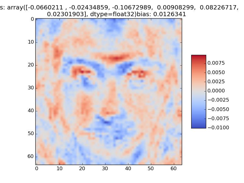
Select two of the actors, and visualize the weights of the hidden units that are useful for classifying input photos as those particular actors. Explain how you selected the hidden units.
A sample visualization is below.
Part 10 (20 pts)
PyTorch comes with an implementation of AlexNet, along with its weights. Extract the values of the activations of AlexNet on the face images in a particular layer (e.g., Conv4). In your report, explain how you did that. Use those as features in order to perform face classification: learn a fully-connected neural network that takes in the activations of the units in the AlexNet layer as inputs, and outputs the name (or index, or one-hot encoding – up to you) of the actor. In your report, include a description of the system you built and its performance, similarly to Part 8. It is possible to improve on the results of Part 8 by reducing the error rate by at least 30%. We recommend starting out with only using the conv4 activations.
PyTorch’s implementation allows you to fairly easily access the layer just before the fully connected layer. You can modify that implementation to access any layer. We include a slightly-modified version of PyTorch’s AlexNet implementation here:
Note that you are asked to only train the (newly-constructed) fully-connected layers on top of the layer that you extracted. In your report, state how you accomplish that.
What to submit
The project should be implemented using Python 2 or 3 and should be runnable on the CS Teaching Labs computers. Your report should be in PDF format. You should use LaTeX to generate the report, and submit the .tex file as well. A sample template is on the course website. You will submit at least the following files: faces.py, digits.py, deepfaces,py, deepnn.tex, and deepnn.pdf. You may submit more files as well. You may submit ipynb files in place of py files.
Reproducibility counts! We should be able to obtain all the graphs and figures in your report by running your code. The only exception is that you may pre-download the images (what and how you did that, including the code you used to download the images, should be included in your submission.) Submissions that are not reproducible will not receive full marks. If your graphs/reported numbers cannot be reproduced by running the code, you may be docked up to 20%. (Of course, if the code is simply incomplete, you may lose even more.) Suggestion: if you are using randomness anywhere, use numpy.random.seed().
You must use LaTeX to generate the report. LaTeX is the tool used to generate virtually all technical reports and research papers in machine learning, and students report that after they get used to writing reports in LaTeX, they start using LaTeX for all their course reports. In addition, using LaTeX facilitates the production of reproducible results.
Available code
You are free to use any of the code available from the CSC411 course website.
Readability
Readability counts! If your code isn’t readable or your report doesn’t make sense, they are not that useful. In addition, the TA can’t read them. You will lose marks for those things.
Academic integrity
It is perfectly fine to discuss general ideas with other people, if you acknowledge ideas in your report that are not your own. However, you must not look at other people’s code, or show your code to other people, and you must not look at other people’s reports and derivations, or show your report and derivations to other people. All of those things are academic offences.