The following experiments were conducted to study the performance of MCVQ as the number of vector quantizers (VQ's) and number of vectors per VQ are varied.
The experiments were carrired out on two data sets of gray-scale images, the first depicting geometric shapes and the second depicting faces.
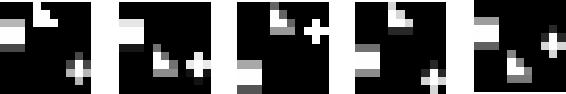
The shapes data set consists of 11-by-11 pixel images, as depicted below. Each image contains three shapes, with fixed horizontal position, but variable vertical position. Since each shape is roughly 3-by-3 pixels, there are 9^3=729 different shape images possible, if each shape must lie on a pixel boundary. These images were enumerated, then each shape was `jittered' vertically by a random value, uniformly distributed between -1 and +1 pixels. Anti-aliasing was employed to render shapes not lying exactly on pixel boundaries.
The training set consisted of 100 of these images, randomly selected. The remaining 629 images comprised the testing set.
The faces data employed was the CBCL FACE DATABASE #1, made available by the MIT Center For Biological and Computation Learning. It consists of 19-by-19 pixel images, each containing a single frontal or near-frontal face. A training set of 1800 images, and a testing set of 629 images was chosen. (This was the same split used for the Multiple Cause Vector Quantization paper.)
Performance at reconstructing the training images was evaluated with the number of VQ's, K, ranging from 1 to 12, and the number of vectors per VQ, J, also ranging from 1 to 12.
For each pair (J,K), an MCVQ model was trained. Convergence of EM was assumed when the free energy had not changed by more than 1e-3 % during the previous three iterations.
For each testing image, the expected values of the latent variables (m's) were inferred. These values were used, with the learned model, to generate a reconstruction of the image. The root-mean-squared error between the reconstruction and the original was calculated, and summed over all the training images.
To smooth out the effects of converging to a local minimum, the above experiment was repeated 10 times for each (J,K).
Annealing was employed for the learning of the m's and the g's, using the schedule: {3, 2.7, 2.4, 2.1, 1.8, 1.5, 1.2, 1, 1, 1, ...}.
As above, with the following differences: