Now we will try to parallerize the process in the previous section.
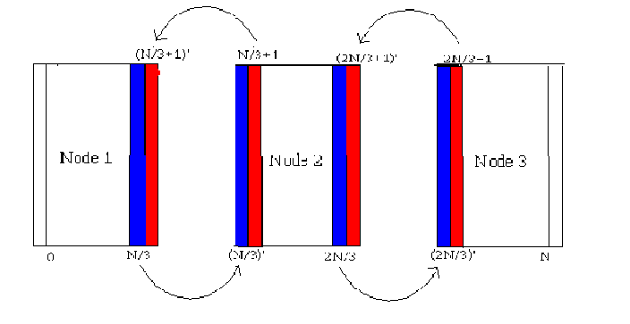
Figure 3.2 shows the strategy to parallelize the algorithm. The values on the outside of each nodes are actually repeated values at the borders divided domain. Before each processor goes and computes its share in each iteration, the processors exchange the border values so that they can be used to compute the accurate values of the next time step in the domain that it is responsible for.
The program takes two command line arguments, one for setting the number of time steps to be computed, and another for setting the square grid size in the domain.
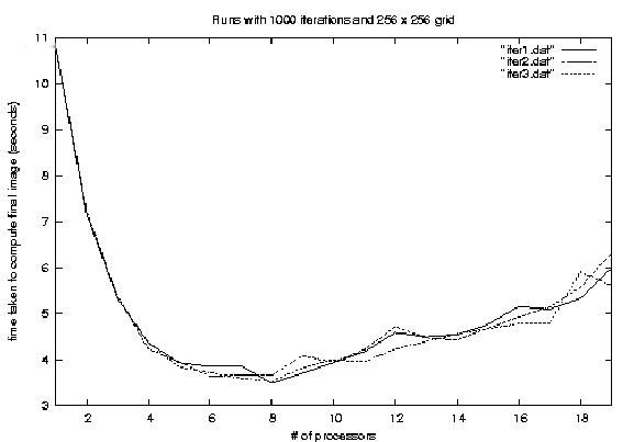
The result depended on which part of the problem domain the "bottleneck" was. Recall that transient heat transfer on a given domain also required the number of time steps to be computed. so if 10,000 iterations were required, then each processor had to do 10,000 iterations no matter what. As it can be seen from the presentation of the results, the time that was saved by adding another processor was greatly reduced due to the amount of communication that has to take place amongst the processors. In fact, figure 3.3 shows the result of running from 1 processor to 19 processors 3 times. It clearly shows that the communication cost overweighs the advantages of increasing the number of processors to work on the problem.
The result for the 2000 time steps may look deceiving. With more iterations, there should be more overhead than the runs with 1000 time steps. Given the stochastic elements of the computer networks, we cannot be sure of exactly what causes this amount of bounce backs with either 1000 time steps and 2000 time steps. However, both runs have 19 processors running approximately 2 seconds slower than the peak speeds. But one thing is sure, as the number of processors increased, the CPU load of a sample processor running the code consistently decreased, indicating the processors did not have as much to do as much as waiting and sending data between processors.
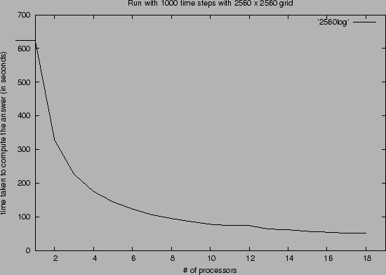
The picture looks a little clearer when we look at the result of the run with much larger grid as we can see in figure 3.5. Now that the problem domain is bigger, the running time consistently decreased as the number of processors increased. So clearly, running the experiments with the same type of an environment, the comparatively large number of time steps as opposed to the domain grid size does make a difference in balancing out the amount of communications that has to take place and the amount of work that each processor has to do.