Introduction


This manual is a reference for using the BTSVQ software. BTSVQ is a computational tool to analyze and visualize microarray gene expression data. BTSVQ clustering and visualizing methodology is given in Sultan at el. The software requires Matlab version 6.0 release 12.1. BTSVQ uses SOM toolbox for computing Self-Organizing Maps and visualization of the data. The SOM toolbox can be found at http://www.cis.hut.fi/projects/somtoolbox/.

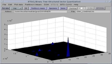
First time users, please follow following analysis steps:

Load data à Plot data à Apply normalizationà Plot data, if required normalize again, or select another normalization, and plot data à Select “Specimens” or “Gene” tab to decide which space you are going to cluster à Decide SOM topology, or press topology tab for software to suggest topology. à Compute SOM, if the component planes are not visually distinguishable and are homogenous, select some different topology or do other normalization, and repeat all the above steps.à Press “Partitive k-means” tab for partitive clustering. à Finally hit “BTSVQ” tab to generate clustering results.

All the steps can be repeated in any order, after completing first round, except BTSVQ. To generate another set of results “Partitive k-means” tab should pressed before “BTSVQ”.

Figure (1)
2. Loading Data


BTSVQ offers an easy interface to load data in several different formats. There is no limit to the number of rows and columns in the data.

figure (2)

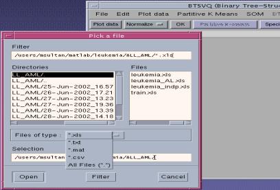
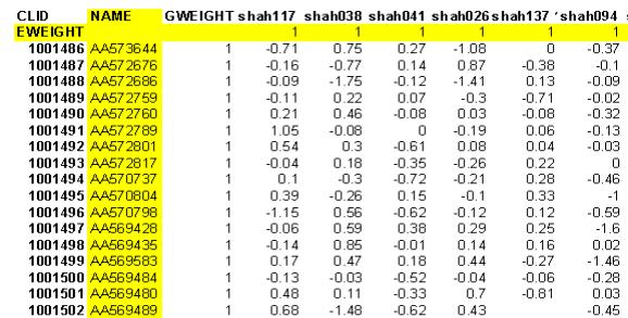
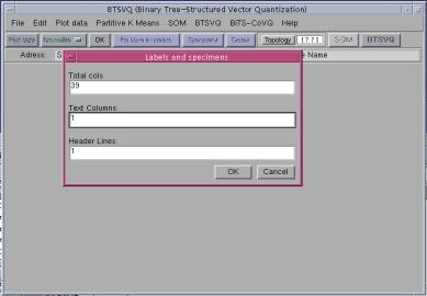
Following file formats are supported.

2.1 ASCII text files

A typical Microarray text file is shown in the Figure (3), First row and first column are taken as the specimen labels and gene labels respectively. The file with more than one row or columns of the descriptors of gene labels or specimen labels can also be loaded. You will be asked of the total number of columns in the text file. Also you will be prompted for the number of gene label columns and specimen label rows in the file, and only first row and first columns will be taken as Specimen label and Gene ID, the rest of the header lines will be discarded, and the data will be loaded beyond that range, as shown in figure (3), the yellow lines will not be included in the analysis.

To load ASCII text files, total number of columns in the file and number of text columns and header lines should be specified.
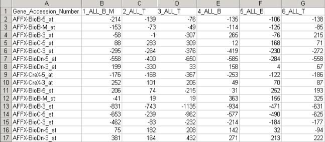
Figure(4)

2.2 Microsoft Excel files

The preferred format of the excel files is shown in Figure (5). If there are more than one text columns or rows for gene ID’s and specimen labels, only first row and column will be considered in the analysis and the rest would be discarded. Also note that specimen and gene labels should be text or Alphanumeric, numeric entries should be changed to alphanumeric. Column A, and Row 1 should have text in it otherwise an XLS read error will appear.

Figure(5)

2.3 Comma Separated (CSV) files.

Coma separated files are also loaded like text files, by specifying total number of columns in the file and number of text columns and header lines.

2.4 Matlab .mat format files

Mat files with following variables present can also be loaded

  • cnames

    Cell strings of specimen names; size = (no_of_specimens X 1)

  • labels

    Cell strings of Gene ID's column; size = (no_of_genes X 1)

  • data

    Matrix; size = (no_of_genes x no_of_samples)

    or

    sD(SOM data-struct) Information about SOM data structs can be found at http://www.cis.hut.fi/projects/somtoolbox/.

    If the mat file is saved using the GUI, it automatically save above listed variables.

    Note:

    If the numbers of specified columns exceed the columns in the data file, empty columns will be added to the data.


3. Plotting the Data

cDNA Microarray data are log ratios of intensities. It is very important to have some visual look of the data before applying any clustering or normalization technique. Surface plots of data offer good visualization of gene expression data in three dimensions. Some times due to outliers, or some very high ratios in the data makes it very skewed, as shown in the figure (6), the raw data has some very high values and rest of the data is more or less uniform. Any clustering method applied on such data will be biased towards the high values.

Figure(6)

Figure(7)


4. Data Normalization

Normalizations are used to transform data to remove various types of noise, biases and outliers. This often results in a new range of the data that is easier to work with in further analysis. The transformation may introduce several distortions and biases, some of which improve the information content, while others may eliminate existing valid patterns. Microarray data is generally log-normalized to provide an equal spread between up and down-regulated genes.

BTSVQ provides three important normalizations, log, variance and range.


5. Partative k-means

Partitive k-menas is splitting hierarchical clustering method. It starts with the whole data set as a single cluster, which is partitioned into disjoint subsets and , where the inter clusters distance is maximized. The subsets and are further subdivided into and , etc., thus, building a binary tree.

6. SOM

Several techniques have been used to visualize this highly multi-dimensional data. The self-organizing map (SOM) algorithm is an efficient tool for the visualization of multidimensional data. SOMs have previously been shown to be effective for the exploratory analysis of gene expression data. SOMs are neural network algorithms widely used in data analysis and vector quantization. The algorithm is similar to k-means clustering, with the additional constraint that cluster centres are restricted to lie in a two dimensional manifold. SOMs show two main characteristics; they realize a quantization of a high-dimensional space, as other vector quantization techniques such as LBG (Gersho and Gray 1992)and k-means, and they exhibit a topological property which allows one to analyze the ordering of centroids. Component planes of SOMs are the planes of Voronoi Tessellations, each representing a specimen in a microarray experiment. Figure (8) presents quantized gene expression visualizations by component planes of SOM.

Figure (8)

Figure 9, shows component planes of the whole data set.

Figure (9)


7. BTSVQ

BTSVQ merges the results of SOM (genes space), and Partitive k-means (specimen space). The algorithm uses vector quantization and self-organizing capabilities of SOMs in finding significant gene centers in gene space (high dimensionality and large number of clusters), and the effectiveness of k-means in experiment space (medium dimensionality and low number of clusters). The resulting binary tree of specimens with SOM component planes of Specimens at nodes is shown in figure 10.

Figure (10)
8. Output

Output is generated in a subdirectory named after current time (DD-MM-YYY_hh.mm) in the parent directory from where the data file is loaded.

  • LOG file listing the data file name, last “Normalization” applied on data.

  • Partitive clustering results (ptree.txt) file.

  • BTSVQ clustering results. (Children of BTSVQ tree, labeled with the Level and Child)